Cross-Correlation

Cross-correlation is a measure of similarity between two series, typically a time series. It is sometimes called the sliding dot product or sliding inner product.

The cross-correlation implements the following conceptual steps:

Given two signals
- $r (t)$ is the reference signal with bounds $[r_{a}, r_{b}]$ .
- $s (t)$ is the subject signal with bounds $[s_{a}, s_{b}]$ .
Synchronization:
- Find the global minimum $T_{a} = min (r_{a}, s_{a})$ .
- Find the global maximum $T_{b} = max (r_{b}, s_{b})$ .
- Construct a global time interval $[T_{a}, T_{b}]$ .
- Choose a global time step, $Δ T$ , to be the minimum of the reference time step and the subject time step.
Correlation:
- Keep the reference signal stationary. Move the subject signal along the $t$ axis until the last data point of the subject signal is multiplied with the first data point of the reference signal.
- Then, slide the subject signal to the right on the $t$ axis by $Δ T$ , calculating the inner product of the two signals for each $Δ T$ in $[T_{a}, T_{b}]$ .
- Find the largest value of the foregoing inner products, and then for that $Δ T$ step, move the subject curve to align with the reference curve. This will represent the highest correlation between the reference and the signal.

The figio implementation is based on the formulations contained in Terpsma et al.¹, Sections E.2 and E.3 (pages 110 to 121).

Example

Consider the sawtooth examples shown below, recreated from the Anomaly webpage, section Normalized Cross-Correlation with Time Shift.²

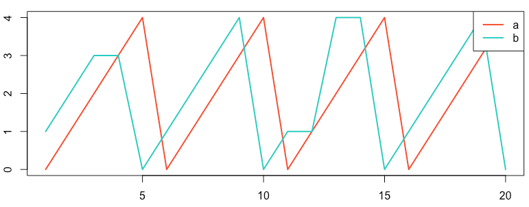
Figure: Reproduction of the sawtooth series on the Anomaly website.²

Create the input file anomaly_recipe.yml

::::::::::::::
anomaly_recipe.yml
::::::::::::::
signal_a:
  type: xymodel
  # folder: ~/autotwin/figio/book/cross_correlation
  folder: ./  # the current directory
  file: signal_a.csv
  skip_rows: 1
  ycolumn: 1
  plot_kwargs:
    label: reference signal a
    color: red
    linewidth: 3
    linestyle: "--"
    marker: D
    alpha: 0.9
signal_b:
  type: xymodel
  # folder: ~/autotwin/figio/book/cross_correlation
  folder: ./  # the current directory
  file: signal_b.csv
  skip_rows: 1
  ycolumn: 1
  plot_kwargs:
    label: subject signal b
    color: darkcyan
    linewidth: 1
    linestyle: "-"
    marker: o
    alpha: 0.8
signal_b_correlated:
  type: xymodel
  # folder: ~/autotwin/figio/book/cross_correlation
  folder: ./  # the current directory
  file: signal_b.csv
  skip_rows: 1
  ycolumn: 1
  plot_kwargs:
    label: subject signal b
    color: darkcyan
    linewidth: 1
    linestyle: "-"
    marker: o
    alpha: 0.8
  signal_process:
    process1:
      correlation:
        reference:
          # folder: ~/autotwin/figio/book/cross_correlation
          folder: ./  # the current directory
          file: signal_a.csv
          skip_rows: 1
          ycolumn: 1
        verbose: true
        serialize: false
        # folder: ~/autotwin/figio/book/cross_correlation
        folder: ./  # the current directory
        file: out_signal_b_correlated.csv
figure_1:
  type: xyview
  model_keys: [ signal_a, signal_b ]
  # folder: ~/autotwin/figio/book/cross_correlation
  folder: ./  # the current directory
  file: out_anomaly_pre_corr.svg
  title: Anomaly site example, pre-correlation
  xlabel: time (s)
  ylabel: position (m)
  xlim: [ -1, 22 ]
  ylim: [ -1, 5 ]
  size: [ 8.0, 6.0 ]
  dpi: 100
  display: true
  details: false
  serialize: true
figure_2:
  type: xyview
  model_keys: [ signal_a, signal_b_correlated ]
  # folder: ~/autotwin/figio/book/cross_correlation
  folder: ./  # the current directory
  file: out_anomaly_post_corr.svg
  title: Anomaly site example, post-correlation
  xlabel: time (s)
  ylabel: position (m)
  xlim: [ -1, 22 ]
  ylim: [ -1, 5 ]
  size: [ 8.0, 6.0 ]
  dpi: 100
  display: true
  details: false
  serialize: true

which makes use of the two data series signal_a.csv and signal_b.csv.

::::::::::::::
signal_a.csv
::::::::::::::
time (s),signal_a (m)
1,0
2,1
3,2
4,3
5,4
6,0
7,1
8,2
9,3
10,4
11,0
12,1
13,2
14,3
15,4
16,0
17,1
18,2
19,3
20,4

::::::::::::::
signal_b.csv
::::::::::::::
time (s),signal_b (m)
1,1
2,2
3,3
4,3
5,0
6,1
7,2
8,3
9,4
10,0
11,1
12,1
13,4
14,4
15,0
16,1
17,2
18,3
19,4
20,0

Results

Run figio on the input file to produce the figures.

figio anomaly_receipe.yml

Processing file: anomaly_recipe.yml
====================================
Information
For (x, y) data and time series data:
  type: xymodel items associate with type: xyview items.
For histogram data:
  type: hmodel items associate with type: hview items.
====================================

This is xymodel.cross_correlation...
reference: [[ 1.  0.]
 [ 2.  1.]
 [ 3.  2.]
 [ 4.  3.]
 [ 5.  4.]
 [ 6.  0.]
 [ 7.  1.]
 [ 8.  2.]
 [ 9.  3.]
 [10.  4.]
 [11.  0.]
 [12.  1.]
 [13.  2.]
 [14.  3.]
 [15.  4.]
 [16.  0.]
 [17.  1.]
 [18.  2.]
 [19.  3.]
 [20.  4.]]
subject: [[ 1.  1.]
 [ 2.  2.]
 [ 3.  3.]
 [ 4.  3.]
 [ 5.  0.]
 [ 6.  1.]
 [ 7.  2.]
 [ 8.  3.]
 [ 9.  4.]
 [10.  0.]
 [11.  1.]
 [12.  1.]
 [13.  4.]
 [14.  4.]
 [15.  0.]
 [16.  1.]
 [17.  2.]
 [18.  3.]
 [19.  4.]
 [20.  0.]]

Synchronization...
  Reference [t_min, t_max] by dt (s): [1.0, 20.0] by 1.0
  Subject [t_min, t_max] by dt (s): [1.0, 20.0] by 1.0
  Globalized [t_min, t_max] by dt (s): [1.0, 20.0] by 1.0
  Globalized times: [ 1.  2.  3.  4.  5.  6.  7.  8.  9. 10. 11. 12. 13. 14. 15. 16. 17. 18.
 19. 20.]
  Length of globalized times: 20

Correlation...
  Sliding dot product (cross-correlation): [  0.   0.   4.  11.  20.  30.  20.  19.  27.  41.  61.  41.  30.  42.
  61.  91.  61.  44.  55.  78. 117.  81.  51.  48.  58.  87.  61.  36.
  32.  37.  56.  40.  25.  17.  17.  26.  20.  11.   4.]
  Length of the sliding dot product: 39
  Max sliding dot product (cross-correlation): 117.0
  Sliding dot product of normalized signals (cross-correlation): [0.         0.         0.03375798 0.09283444 0.16878989 0.25318484
 0.16878989 0.1603504  0.22786636 0.34601928 0.51480918 0.34601928
 0.25318484 0.35445878 0.51480918 0.76799402 0.51480918 0.37133777
 0.46417221 0.65828059 0.98742088 0.68359907 0.43041423 0.40509575
 0.48949069 0.73423604 0.51480918 0.30382181 0.27006383 0.3122613
 0.4726117  0.33757979 0.21098737 0.14347141 0.14347141 0.21942686
 0.16878989 0.09283444 0.03375798]
  Correlated time_shift (from full left)=20.0
  Correlated index_shift (from full left)=20
  Correlated time step (s): 1.0
  Correlated t_min (s): 1.0
  Correlated t_max (s): 21.0
  Correlated times: [ 1.  2.  3.  4.  5.  6.  7.  8.  9. 10. 11. 12. 13. 14. 15. 16. 17. 18.
 19. 20. 21.]
  Correlated reference f(t): [0. 1. 2. 3. 4. 0. 1. 2. 3. 4. 0. 1. 2. 3. 4. 0. 1. 2. 3. 4. 0.]
  Correlated subject f(t): [0. 1. 2. 3. 3. 0. 1. 2. 3. 4. 0. 1. 1. 4. 4. 0. 1. 2. 3. 4. 0.]
  Correlated error f(t): [ 0.  0.  0.  0. -1.  0.  0.  0.  0.  0.  0.  0. -1.  1.  0.  0.  0.  0.
  0.  0.  0.]
  reference_self_correlation: 120.0
  cross_correlation: 117.0
    >> cross_correlation_relative_error=0.025
    >> L2-norm error rate: 0.08247860988423225
  Signal process "correlation" completed.
Finished XYViewBase constructor.
Finished XYViewBase constructor.
Creating view with guid = "figure_1"
  Adding ['signal_a', 'signal_b'] model(s) to current view.
  Figure dpi set to 100
  Figure size set to [8.0, 6.0] inches.
  Serialized view to: out_anomaly_pre_corr.svg
Creating view with guid = "figure_2"
  Adding ['signal_a', 'signal_b_correlated'] model(s) to current view.
  Figure dpi set to 100
  Figure size set to [8.0, 6.0] inches.
  Serialized view to: out_anomaly_post_corr.svg
====================================
End of figio execution.

Error metrics:

cross-correlation relative error: 2.5 percent
L2-norm error rate: 8.3 percent

References

Terpsma RJ, Hovey CB. Blunt impact brain injury using cellular injury criterion. Sandia National Lab. (SNL-NM), Albuquerque, NM (United States); 2020 Oct 1. link

Understanding Cross-Correlation, Auto-Correlation, Normalization and Time Shift, March 8, 2016. Available from: https://anomaly.io/understand-auto-cross-correlation-normalized-shift/