Introduction

figio is Python application that uses declarative yml input file recipes to produce high quality matplotlib and $\text{LATEX}$ figures.

The following figure types are currently supported:

• (x, y) data (or, equivalently, time series data), and
• histogram data.

Installation

Use of a virtual environment is recommended but not necessary.

python -m venv .venv

# Activate the venv with one of the following:
source .venv/bin/activate       # for bash shell
source .venv/bin/activate.csh   # for c shell
source .venv/bin/activate.fish  # for fish shell
.\.venv\Scripts\activate        # for powershell

Install figio from the Python Package Index (PyPI).

pip install figio

Getting Started

Tabular data is used as the data source of figio figures. Let's get started with a tabular data for the inflation rate, measured on the first day or each year. The tabular data, inflation.csv, comes from the Federal Reserve Bank of St. Louis.

::::::::::::::
inflation.csv
::::::::::::::
observation_date,FPCPITOTLZGUSA
1960,1.457975986277910
1961,1.070724147647240
1962,1.198773348201860
1963,1.239669421487530
1964,1.278911564625910
1965,1.585169263836620
1966,3.015075376884400
1967,2.772785622593090
1968,4.271796152885370
1969,5.462386200287450
1970,5.838255338482510
1971,4.292766688130510
1972,3.272278246552830
1973,6.177760063770380
1974,11.054804804804800
1975,9.143146864965351
1976,5.744812635490850
1977,6.501683994728400
1978,7.630963838856060
1979,11.254471129279500
1980,13.549201974968399
1981,10.334715340277100
1982,6.131427000274930
1983,3.212435233160650
1984,4.300535475234290
1985,3.545644152093650
1986,1.898047722342760
1987,3.664563217516900
1988,4.077741107444130
1989,4.827003030089440
1990,5.397956439903250
1991,4.234963964538490
1992,3.028819678149690
1993,2.951656966385590
1994,2.607441592154530
1995,2.805419688536620
1996,2.931204199934410
1997,2.337689937307350
1998,1.552279098743640
1999,2.188027196973580
2000,3.376857271499290
2001,2.826171118854070
2002,1.586031626506010
2003,2.270094973361150
2004,2.677236693091720
2005,3.392746845495500
2006,3.225944100704040
2007,2.852672481501380
2008,3.839100296651000
2009,-0.355546266299747
2010,1.640043442389900
2011,3.156841568622000
2012,2.069337265260670
2013,1.464832655627170
2014,1.622222977408170
2015,0.118627135552451
2016,1.261583205705360
2017,2.130110003659610
2018,2.442583296928170
2019,1.812210075260210
2020,1.233584396306290
2021,4.697858863637420
2022,8.002799820521210
2023,4.116338383744880

To plot this data, we create a yml input file called inflation.yml.

::::::::::::::
inflation.yml
::::::::::::::
inflation-data:
  type: xymodel
  folder: ./  # the current directory
  file: inflation.csv
  skip_rows: 1
  plot_kwargs:
    label: inflation rate
    linestyle: "-"  # solid line
    linewidth: 1.0
    marker: "."  # point marker
  ycolumn: 1
inflation-figure:
  type: xyview
  folder: ./  # the current directory
  file: inflation.svg  # the output file
  size: [ 8.0, 6.0 ]
  title: Inflation, consumer prices for the United States (FPCPITOTLZGUSA)
  xlabel: year
  ylabel: inflation rate (%)
  details: false
  display: true
  dpi: 100
  latex: false
  serialize: true

Run figio on the input file to produce the figure:

figio inflation.yml

Processing file: inflation.yml
====================================
Information
For (x, y) data and time series data:
  type: xymodel items associate with type: xyview items.
For histogram data:
  type: hmodel items associate with type: hview items.
====================================
Finished XYViewBase constructor.
Creating view with guid = "inflation-figure"
  Adding all models to current view.
  Figure dpi set to 100
  Figure size set to [8.0, 6.0] inches.
  Serialized view to: inflation.svg
====================================
End of figio execution.

The following figure appears:

Congratulations! You just make your first figio figure.

Keys and Values

Below are dictionary key: value pairs, followed by a description, for each of the figio dictionary constitutents.

Main figio Dictionary

The figio dictionary is the main dictionary.

• It is stored in an ordinary text file in yml format.
• It is composed of one or more model dictionaries and one or more view dictionaries.

There are three common variations to the figio dictionary:

• 1:1
  • One model
  • One view
  • This is the most basic option.
• 1:n
  • Several models
  • One view
  • This is an advanced option, wherein multiple models are plotted to the same figure. Considerations such as y-axis limits or the possibility of dual y-axes can become important.
• m:n
  • Several models
  • Several views
  • This is the most advanced combination of the three, where all the models are created, and views explicity specify which models get plotted to a particular figure.

Signal processing may be performed on one or more models, using the signal_process dictionary, to create a new model, which can also be used by the view. A conceptual flow diagram of multiple models, one with signal processing, and one view is shown below.

┌───────────────┐                                                    ┌───────────────┐
│     Model     │─────────────────────────┐                          │               │
└───────────────┘                         │                          │               │
                                          │                          │               │
┌───────────────┐                         │                          │               │
│     Model     │─────────────────────────┤                          │               │
└───────────────┘                         │                          │               │
        │                                 │                          │     View      │
                                          ├─────────────────────┬───▶│               │
        │                                 │                     │    │               │
┌───────────────┐                         │                     │    │               │
│     Model     │──┬──────────────────────┘                     │    │               │
└───────────────┘  │   ┌───────────────┐                        │    │               │
                   │   │    Signal     │    ┌───────────────┐   │    │               │
                   └──▶│    Process    │───▶│     Model     │───┘    │               │
                       └───────────────┘    └───────────────┘        └───────────────┘

Model Dictionary

The model dictionary contains items that describe how each (x,y) data set is constructed and shown on the view.

Plot Keywords Dictionary

Dictionary that overrides the matplotlib.pyplot.plot() kwargs default values. Default values used by figio follow:

Signal Processing Keywords Dictionary

Warning: The Signal Processing dictionary and links below are a work in progress.

This dictionary is currently under active development. For additional documentation, see

• Butterworth filter
• Differentiation
• Integration
• Cross correlation (to come, not yet implemented)
• tpav (three points angular velocity) algorithm

Below is a summary of the key: value pairs available within the signal_process dictionary.

        signal_process:
            process_guid_1:
                butterworth:
                    cutoff: 5
                    order: 4
                    type: low
            process_guid_2:
                gradient:
                    order: 1
            process_guid_3:
                integration:
                    order: 3
                    initial_conditions: [-10, 100, 1000]
            process_guid_4:
                crosscorrelation:
                    model_keys: [model_guid_0, model_guid_1]
                    mode: full # (valid | same)
            process_guid_5:
                tpav: { (tpav is three points angular velocity)
                    model_keys: [model_guid_0, model_guid_1, model_guid_2]

All processes support serialization, via

        signal_process:
            process_guid:
                process_key_string:
                    serialize: 1
                    folder: ~/sibl/cli/io/example
                    file: processed_output_file.csv

View Dictionary

The view dictionary contains items that describe how the main figure is constructed.

yaxis_rhs Dictionary

background_image Dictionary

Multiple Series

We show an examples of multiple series using default and non-default values for the line specifications (color, transparency, type).

The file data.csv contains colums for time (s),sin(t),cos(2t).

::::::::::::::
data.csv
::::::::::::::
time (s),sin(t),cos(2t)
0,0,1
0.1,0.099833417,0.980066578
0.2,0.198669331,0.921060994
0.3,0.295520207,0.825335615
0.4,0.389418342,0.696706709
0.5,0.479425539,0.540302306
0.6,0.564642473,0.362357754
0.7,0.644217687,0.169967143
0.8,0.717356091,-0.029199522
0.9,0.78332691,-0.227202095
1,0.841470985,-0.416146837
1.1,0.89120736,-0.588501117
1.2,0.932039086,-0.737393716
1.3,0.963558185,-0.856888753
1.4,0.98544973,-0.942222341
1.5,0.997494987,-0.989992497
1.6,0.999573603,-0.998294776
1.7,0.99166481,-0.966798193
1.8,0.973847631,-0.896758416
1.9,0.946300088,-0.790967712
2,0.909297427,-0.653643621
2.1,0.863209367,-0.490260821
2.2,0.808496404,-0.30733287
2.3,0.745705212,-0.112152527
2.4,0.675463181,0.087498983
2.5,0.598472144,0.283662185
2.6,0.515501372,0.468516671
2.7,0.42737988,0.634692876
2.8,0.33498815,0.775565879
2.9,0.239249329,0.885519517
3,0.141120008,0.960170287
3.1,0.041580662,0.996542097
3.2,-0.058374143,0.993184919
3.3,-0.157745694,0.950232592
3.4,-0.255541102,0.86939749
3.5,-0.350783228,0.753902254
3.6,-0.442520443,0.608351315
3.7,-0.529836141,0.438547328
3.8,-0.611857891,0.251259843
3.9,-0.687766159,0.053955421
4,-0.756802495,-0.145500034
4.1,-0.818277111,-0.339154861
4.2,-0.871575772,-0.519288654
4.3,-0.916165937,-0.678720047
4.4,-0.951602074,-0.811093014
4.5,-0.977530118,-0.911130262
4.6,-0.993691004,-0.974843621
4.7,-0.999923258,-0.999693042
4.8,-0.996164609,-0.984687856
4.9,-0.982452613,-0.930426272
5,-0.958924275,-0.839071529
5.1,-0.925814682,-0.714265652
5.2,-0.883454656,-0.560984257
5.3,-0.832267442,-0.385338191
5.4,-0.772764488,-0.194329906
5.5,-0.705540326,0.004425698
5.6,-0.631266638,0.203004864
5.7,-0.550685543,0.393490866
5.8,-0.464602179,0.56828963
5.9,-0.373876665,0.720432479
6,-0.279415498,0.843853959
6.1,-0.182162504,0.933633644
6.2,-0.083089403,0.986192302
6.3,0.0168139,0.999434586

To plot this data, we create a yml input file called recipe.yml.

::::::::::::::
recipe.yml
::::::::::::::
sine-data:
  type: xymodel
  folder: ./  # the current directory
  file: data.csv
  skip_rows: 1
  plot_kwargs:
    label: sin(t)
    color: darkorange
    linestyle: "-"
    linewidth: 4
    alpha: 0.5
cosine-data:
  type: xymodel
  folder: ./  # the current directory
  file: data.csv
  skip_rows: 1
  ycolumn: 2
  plot_kwargs:
    label: cos(2t)
    linestyle: "-."
    linewidth: 2
figure:
  type: xyview
  folder: ./  # the current directory
  file: recipe.svg
  size: [ 8.0, 6.0 ]
  title: Example using figio
  xlabel: time (s)
  ylabel: functions of time f(t)
  yaxis_rhs:
    scale: 10
    label: right-hand-side label with 10 f(t) scale
    yticks: [ -10, -5, 0, 5, 10 ]
  details: false
  display: true
  dpi: 100
  latex: false
  serialize: true

Run figio on the input file to produce the figure:

figio recipe.yml

Processing file: recipe.yml
====================================
Information
For (x, y) data and time series data:
  type: xymodel items associate with type: xyview items.
For histogram data:
  type: hmodel items associate with type: hview items.
====================================
Finished XYViewBase constructor.
Creating view with guid = "figure"
  Adding all models to current view.
  Figure dpi set to 100
  Figure size set to [8.0, 6.0] inches.
  Serialized view to: recipe.svg
====================================
End of figio execution.

The following figure appears:

Congratulations! You just made a figio figure with two data sources.

Cross-Correlation

Cross-correlation is a measure of similarity between two series, typically a time series. It is sometimes called the sliding dot product or sliding inner product.

The cross-correlation implements the following conceptual steps:

• Given two signals
  • $r(t)$ is the reference signal with bounds $[r_a,r_b]$.
  • $s(t)$ is the subject signal with bounds $[s_a,s_b]$.
• Synchronization:
  • Find the global minimum $T_a=\min (r_a,s_a)$.
  • Find the global maximum $T_b=\max (r_b,s_b)$.
  • Construct a global time interval $[T_a,T_b]$.
  • Choose a global time step, $\Delta T$, to be the minimum of the reference time step and the subject time step.
• Correlation:
  • Keep the reference signal stationary. Move the subject signal along the $t$ axis until the last data point of the subject signal is multiplied with the first data point of the reference signal.
  • Then, slide the subject signal to the right on the $t$ axis by $\Delta T$, calculating the inner product of the two signals for each $\Delta T$ in $[T_a,T_b]$.
  • Find the largest value of the foregoing inner products, and then for that $\Delta T$ step, move the subject curve to align with the reference curve. This will represent the highest correlation between the reference and the signal.

The figio implementation is based on the formulations contained in Terpsma et al.¹, Sections E.2 and E.3 (pages 110 to 121).

Example

Consider the sawtooth examples shown below, recreated from the Anomaly webpage, section Normalized Cross-Correlation with Time Shift.²

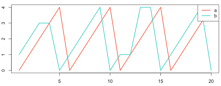
Figure: Reproduction of the sawtooth series on the Anomaly website.²

Create the input file anomaly_recipe.yml

::::::::::::::
anomaly_recipe.yml
::::::::::::::
signal_a:
  type: xymodel
  # folder: ~/autotwin/figio/book/cross_correlation
  folder: ./  # the current directory
  file: signal_a.csv
  skip_rows: 1
  ycolumn: 1
  plot_kwargs:
    label: reference signal a
    color: red
    linewidth: 3
    linestyle: "--"
    marker: D
    alpha: 0.9
signal_b:
  type: xymodel
  # folder: ~/autotwin/figio/book/cross_correlation
  folder: ./  # the current directory
  file: signal_b.csv
  skip_rows: 1
  ycolumn: 1
  plot_kwargs:
    label: subject signal b
    color: darkcyan
    linewidth: 1
    linestyle: "-"
    marker: o
    alpha: 0.8
signal_b_correlated:
  type: xymodel
  # folder: ~/autotwin/figio/book/cross_correlation
  folder: ./  # the current directory
  file: signal_b.csv
  skip_rows: 1
  ycolumn: 1
  plot_kwargs:
    label: subject signal b
    color: darkcyan
    linewidth: 1
    linestyle: "-"
    marker: o
    alpha: 0.8
  signal_process:
    process1:
      correlation:
        reference:
          # folder: ~/autotwin/figio/book/cross_correlation
          folder: ./  # the current directory
          file: signal_a.csv
          skip_rows: 1
          ycolumn: 1
        verbose: true
        serialize: false
        # folder: ~/autotwin/figio/book/cross_correlation
        folder: ./  # the current directory
        file: out_signal_b_correlated.csv
figure_1:
  type: xyview
  model_keys: [ signal_a, signal_b ]
  # folder: ~/autotwin/figio/book/cross_correlation
  folder: ./  # the current directory
  file: out_anomaly_pre_corr.svg
  title: Anomaly site example, pre-correlation
  xlabel: time (s)
  ylabel: position (m)
  xlim: [ -1, 22 ]
  ylim: [ -1, 5 ]
  size: [ 8.0, 6.0 ]
  dpi: 100
  display: true
  details: false
  serialize: true
figure_2:
  type: xyview
  model_keys: [ signal_a, signal_b_correlated ]
  # folder: ~/autotwin/figio/book/cross_correlation
  folder: ./  # the current directory
  file: out_anomaly_post_corr.svg
  title: Anomaly site example, post-correlation
  xlabel: time (s)
  ylabel: position (m)
  xlim: [ -1, 22 ]
  ylim: [ -1, 5 ]
  size: [ 8.0, 6.0 ]
  dpi: 100
  display: true
  details: false
  serialize: true

which makes use of the two data series signal_a.csv and signal_b.csv.

::::::::::::::
signal_a.csv
::::::::::::::
time (s),signal_a (m)
1,0
2,1
3,2
4,3
5,4
6,0
7,1
8,2
9,3
10,4
11,0
12,1
13,2
14,3
15,4
16,0
17,1
18,2
19,3
20,4

::::::::::::::
signal_b.csv
::::::::::::::
time (s),signal_b (m)
1,1
2,2
3,3
4,3
5,0
6,1
7,2
8,3
9,4
10,0
11,1
12,1
13,4
14,4
15,0
16,1
17,2
18,3
19,4
20,0

Results

Run figio on the input file to produce the figures.

figio anomaly_receipe.yml

Processing file: anomaly_recipe.yml
====================================
Information
For (x, y) data and time series data:
  type: xymodel items associate with type: xyview items.
For histogram data:
  type: hmodel items associate with type: hview items.
====================================

This is xymodel.cross_correlation...
reference: [[ 1.  0.]
 [ 2.  1.]
 [ 3.  2.]
 [ 4.  3.]
 [ 5.  4.]
 [ 6.  0.]
 [ 7.  1.]
 [ 8.  2.]
 [ 9.  3.]
 [10.  4.]
 [11.  0.]
 [12.  1.]
 [13.  2.]
 [14.  3.]
 [15.  4.]
 [16.  0.]
 [17.  1.]
 [18.  2.]
 [19.  3.]
 [20.  4.]]
subject: [[ 1.  1.]
 [ 2.  2.]
 [ 3.  3.]
 [ 4.  3.]
 [ 5.  0.]
 [ 6.  1.]
 [ 7.  2.]
 [ 8.  3.]
 [ 9.  4.]
 [10.  0.]
 [11.  1.]
 [12.  1.]
 [13.  4.]
 [14.  4.]
 [15.  0.]
 [16.  1.]
 [17.  2.]
 [18.  3.]
 [19.  4.]
 [20.  0.]]

Synchronization...
  Reference [t_min, t_max] by dt (s): [1.0, 20.0] by 1.0
  Subject [t_min, t_max] by dt (s): [1.0, 20.0] by 1.0
  Globalized [t_min, t_max] by dt (s): [1.0, 20.0] by 1.0
  Globalized times: [ 1.  2.  3.  4.  5.  6.  7.  8.  9. 10. 11. 12. 13. 14. 15. 16. 17. 18.
 19. 20.]
  Length of globalized times: 20

Correlation...
  Sliding dot product (cross-correlation): [  0.   0.   4.  11.  20.  30.  20.  19.  27.  41.  61.  41.  30.  42.
  61.  91.  61.  44.  55.  78. 117.  81.  51.  48.  58.  87.  61.  36.
  32.  37.  56.  40.  25.  17.  17.  26.  20.  11.   4.]
  Length of the sliding dot product: 39
  Max sliding dot product (cross-correlation): 117.0
  Sliding dot product of normalized signals (cross-correlation): [0.         0.         0.03375798 0.09283444 0.16878989 0.25318484
 0.16878989 0.1603504  0.22786636 0.34601928 0.51480918 0.34601928
 0.25318484 0.35445878 0.51480918 0.76799402 0.51480918 0.37133777
 0.46417221 0.65828059 0.98742088 0.68359907 0.43041423 0.40509575
 0.48949069 0.73423604 0.51480918 0.30382181 0.27006383 0.3122613
 0.4726117  0.33757979 0.21098737 0.14347141 0.14347141 0.21942686
 0.16878989 0.09283444 0.03375798]
  Correlated time_shift (from full left)=20.0
  Correlated index_shift (from full left)=20
  Correlated time step (s): 1.0
  Correlated t_min (s): 1.0
  Correlated t_max (s): 21.0
  Correlated times: [ 1.  2.  3.  4.  5.  6.  7.  8.  9. 10. 11. 12. 13. 14. 15. 16. 17. 18.
 19. 20. 21.]
  Correlated reference f(t): [0. 1. 2. 3. 4. 0. 1. 2. 3. 4. 0. 1. 2. 3. 4. 0. 1. 2. 3. 4. 0.]
  Correlated subject f(t): [0. 1. 2. 3. 3. 0. 1. 2. 3. 4. 0. 1. 1. 4. 4. 0. 1. 2. 3. 4. 0.]
  Correlated error f(t): [ 0.  0.  0.  0. -1.  0.  0.  0.  0.  0.  0.  0. -1.  1.  0.  0.  0.  0.
  0.  0.  0.]
  reference_self_correlation: 120.0
  cross_correlation: 117.0
    >> cross_correlation_relative_error=0.025
    >> L2-norm error rate: 0.08247860988423225
  Signal process "correlation" completed.
Finished XYViewBase constructor.
Finished XYViewBase constructor.
Creating view with guid = "figure_1"
  Adding ['signal_a', 'signal_b'] model(s) to current view.
  Figure dpi set to 100
  Figure size set to [8.0, 6.0] inches.
  Serialized view to: out_anomaly_pre_corr.svg
Creating view with guid = "figure_2"
  Adding ['signal_a', 'signal_b_correlated'] model(s) to current view.
  Figure dpi set to 100
  Figure size set to [8.0, 6.0] inches.
  Serialized view to: out_anomaly_post_corr.svg
====================================
End of figio execution.

Error metrics:

• cross-correlation relative error: 2.5 percent
• L2-norm error rate: 8.3 percent

References

Histograms

Given a particular column from a csv data source, figio can create a frequency count histogram. We illustrate this functionality on a large data set called sr2s10.csv (5.4 MB) and sr2s50.csv (11 MB). To reproduce this example, download the two data sets and place them in a local ~/temp folder.

For concreteness in the following discussion, the first 10 rows of sr2s10.csv appear below:

  maximum edge ratio,    minimum scaled jacobian,               maximum skew,                     volume
          1.000000e0,                6.663165e-1,                2.872659e-1,                4.368155e-2
          1.193120e0,                6.478237e-1,                4.187394e-1,                8.360088e-2
          1.247881e0,                6.474025e-1,                4.065007e-1,                9.447332e-2
          1.214427e0,                6.549605e-1,                3.901043e-1,                8.909662e-2
          1.179123e0,                6.668604e-1,                3.859307e-1,                8.359763e-2
          1.171296e0,                6.702009e-1,                3.868204e-1,                8.222564e-2
          1.175480e0,                6.695364e-1,                3.874507e-1,                8.270613e-2
          1.178150e0,                6.694542e-1,                3.873941e-1,                8.308343e-2

To plot this data, we create a yml input file called histogram.yml.

::::::::::::::
histogram.yml
::::::::::::::
s10_aspect:
  type: hmodel
  folder: ~/temp
  file: sr2s10.csv
  skip_rows: 1
  ycolumn: 0
  plot_kwargs:
    alpha: 0.7
    color: blue
    label: sr2s10
    linewidth: 2.0
s10_msj:
  type: hmodel
  folder: ~/temp
  file: sr2s10.csv
  skip_rows: 1
  ycolumn: 1
  plot_kwargs:
    alpha: 0.7
    color: blue
    label: sr2s10
    linewidth: 2.0
s10_skew:
  type: hmodel
  folder: ~/temp
  file: sr2s10.csv
  skip_rows: 1
  ycolumn: 2
  plot_kwargs:
    alpha: 0.7
    color: blue
    label: sr2s10
    linewidth: 2.0
s10_vol:
  type: hmodel
  folder: ~/temp
  file: sr2s10.csv
  skip_rows: 1
  ycolumn: 3
  plot_kwargs:
    alpha: 0.7
    color: blue
    label: sr2s10
    linewidth: 2.0
s50_aspect:
  type: hmodel
  folder: ~/temp
  file: sr2s50.csv
  skip_rows: 1
  ycolumn: 0
  plot_kwargs:
    alpha: 0.7
    color: orange
    label: sr2s50
    linewidth: 2.0
s50_msj:
  type: hmodel
  folder: ~/temp
  file: sr2s50.csv
  skip_rows: 1
  ycolumn: 1
  plot_kwargs:
    alpha: 0.7
    color: orange
    label: sr2s50
    linewidth: 2.0
s50_skew:
  type: hmodel
  folder: ~/temp
  file: sr2s50.csv
  skip_rows: 1
  ycolumn: 2
  plot_kwargs:
    alpha: 0.7
    color: orange
    label: sr2s50
    linewidth: 2.0
s50_vol:
  type: hmodel
  folder: ~/temp
  file: sr2s50.csv
  skip_rows: 1
  ycolumn: 3
  plot_kwargs:
    alpha: 0.7
    color: orange
    label: sr2s50
    linewidth: 2.0
figure_aspect:
  type: hview
  models: [s10_aspect, s50_aspect]
  folder: ./  # the current directory
  file: hist_sr2sx_aspect.svg
  size: [8.0, 6.0]
  title: Maximum Aspect Ratio
  xlabel: Maximum Aspect Ratio
  ylabel: Frequency
  details: true
  display: true
  dpi: 100
  latex: false
  save: true
figure_msj:
  type: hview
  models: [s10_msj, s50_msj]
  folder: ./  # the current directory
  file: hist_sr2sx_msj.svg
  size: [8.0, 6.0]
  title: Minimum Scaled Jacobian
  xlabel: Minimum Scaled Jacobian
  ylabel: Frequency
  details: true
  display: true
  dpi: 100
  latex: false
  save: true
figure_skew:
  type: hview
  models: [s10_skew, s50_skew]
  folder: ./  # the current directory
  file: hist_sr2sx_skew.svg
  size: [8.0, 6.0]
  title: Maximum Skew
  xlabel: Maximum Skew
  ylabel: Frequency
  details: true
  display: true
  dpi: 100
  latex: false
  save: true
figure_vol:
  type: hview
  models: [s10_vol, s50_vol]
  folder: ./  # the current directory
  file: hist_sr2sx_vol.svg
  size: [8.0, 6.0]
  title: Element Volume
  xlabel: Element Volume
  ylabel: Frequency
  details: true
  display: true
  dpi: 100
  latex: false
  save: true

Run figio on the input file to produce the figures:

figio histogram.yml

Processing file: histogram.yml
====================================
Information
For (x, y) data and time series data:
  type: xymodel items associate with type: xyview items.
For histogram data:
  type: hmodel items associate with type: hview items.
====================================
Histogram default plot_kwargs: {'alpha': 1.0, 'bins': 20, 'color': 'black', 'histtype': 'step', 'label': '', 'linewidth': 1.0, 'log': True}
Histogram updated plot_kwargs: {'alpha': 0.7, 'bins': 20, 'color': 'blue', 'histtype': 'step', 'label': 'sr2s10', 'linewidth': 2.0, 'log': True}
Valid: Validated data: {'alpha': 0.7, 'bins': 20, 'color': 'blue', 'histtype': 'step', 'label': 'sr2s10', 'linewidth': 2.0, 'log': True}

The following figures appears:

Development

Client Configuration

pip install figio

Developer Configuration

From the ~/autotwin/figio folder, create the virtual enivronment,

python -m venv .venv
source .venv/bin/activate       # bash
source .venv/bin/activate.fish  # fish shell

Install the code in editable form,

pip install -e .[dev]

Manual Distribution

python -m build . --sdist  # source distribution
python -m build . --wheel
twine check dist/*

Distribution

The distribution steps will tag the code state as a release version, with a semantic version number, build the code as a wheel file, and publish to the wheel file as a release to GitHub.

Tag

View existing tags, if any:

git tag

Create a tag. Tags can be lightweight or annotated. Annotated tags are recommended since they store tagger name, email, date, and message information. Create an annotated tag:

# example of an annotated tag
git tag -a v1.0.0 -m "Release version 1.0.0"

Push the tag to repo

# example continued
git push origin v1.0.0

Verify the tag appears on the repo

Build

Ensure that setuptools and build are installed:

pip install setuptools build

Navigate to the project directory, where the pyproject.toml file is located and create a wheel distribution.

# generates a .whl file in the dist directory
python -m build --wheel

Semantic Version Bump

Create .github/workflows/bump.yml as follows:

name: Bump
on:
  release:
    types: published
jobs:
  bump:
    runs-on: ubuntu-latest
    steps:
      - name: checkout
        uses: actions/checkout@v4
      - name: bump
        id: bump
        run: |
          # VERSION=$(cargo tree | grep automesh | cut -d " " -f 2 | cut -d "v" -f 2)
          VERSION=$(grep version pyproject.toml | cut -d '"' -f 2)
          MAJOR_MINOR=$(echo $VERSION | rev | cut -d "." -f 2- | rev)
          PATCH=$(echo $VERSION | rev | cut -d "." -f 1)
          BUMP=$(( $PATCH + 1))
          BUMPED_VERSION=$(echo $MAJOR_MINOR"."$BUMP)
          BUMP_BRANCH=$(echo "bump-$VERSION-to-$BUMPED_VERSION")
          echo "bump_branch=$BUMP_BRANCH" >> $GITHUB_OUTPUT
          sed -i "s/version = \"$VERSION\"/version = \"$BUMPED_VERSION\"/" pyproject.toml
          git config --global user.email "bump"
          git config --global user.name "bump"
          git add pyproject.toml
          git commit -m "Bumping version from $VERSION to $BUMPED_VERSION."
          git branch $BUMP_BRANCH
          git checkout $BUMP_BRANCH
          git push --set-upstream origin $BUMP_BRANCH
      - name: pr
        uses: rematocorp/open-pull-request-action@v1
        with:
          github-token: ${{ secrets.GITHUB_TOKEN }}
          from-branch: ${{ steps.bump.outputs.bump_branch }}
          to-branch: ${{ github.event.repository.default_branch }}
          repository-owner: autotwin
          repository: ${{ github.event.repository.name }}