Unit Sphere
A sphere is a useful model because, given its radius, the surface area and volume are known quantities. The error of any surface that approximates the analytical surface of the sphere can be easily quantified.
This page builds a unit sphere from a voxel segmentation. Voxels inside the
sphere have value 1. Voxels outside have value 0. Marching cubes turns
the segmentation into a triangulated surface. That surface approximates the
isosurface of the segmentation at the value
0.5, halfway between 0 and 1. We measure the triangulated surface against
the exact sphere.
Related Studies
Two other sections build unit spheres by other methods.
- Octa-Loop, on the Subdivision page, refines a unit octahedron into a sphere by Loop subdivision.
- Remesh: Unit Sphere remeshes a unit sphere of 1,088 facets.
Segmentation
The script unit_sphere_segmentation.py builds
a sphere of radius voxels. The sphere sits at the center of a cube of
voxels per side. A voxel is inside when its center satisfies
. An inside voxel has value 1, and every other
voxel has value 0. The array axes are , the order automesh
reads from a .npy file.
uv run --with numpy unit_sphere_segmentation.py
The script writes five segmentations of increasing resolution: = 10, 20, 40, 80, and 160. Each voxel has side length once the sphere is scaled to radius 1. The volume column counts the inside voxels and multiplies by . The error, , compares that volume with the exact volume .
| grid | total voxels | inside voxels | volume | error | |
|---|---|---|---|---|---|
| 10 | 21×21×21 | 9,261 | 4,169 | 4.1690 | −0.47% |
| 20 | 41×41×41 | 68,921 | 33,401 | 4.1751 | −0.33% |
| 40 | 81×81×81 | 531,441 | 267,761 | 4.1838 | −0.12% |
| 80 | 161×161×161 | 4,173,281 | 2,143,641 | 4.1868 | −0.05% |
| 160 | 321×321×321 | 33,076,161 | 17,155,325 | 4.1883 | −0.01% |
The voxel volume falls short at every in the table, and the shortfall shrinks as grows.
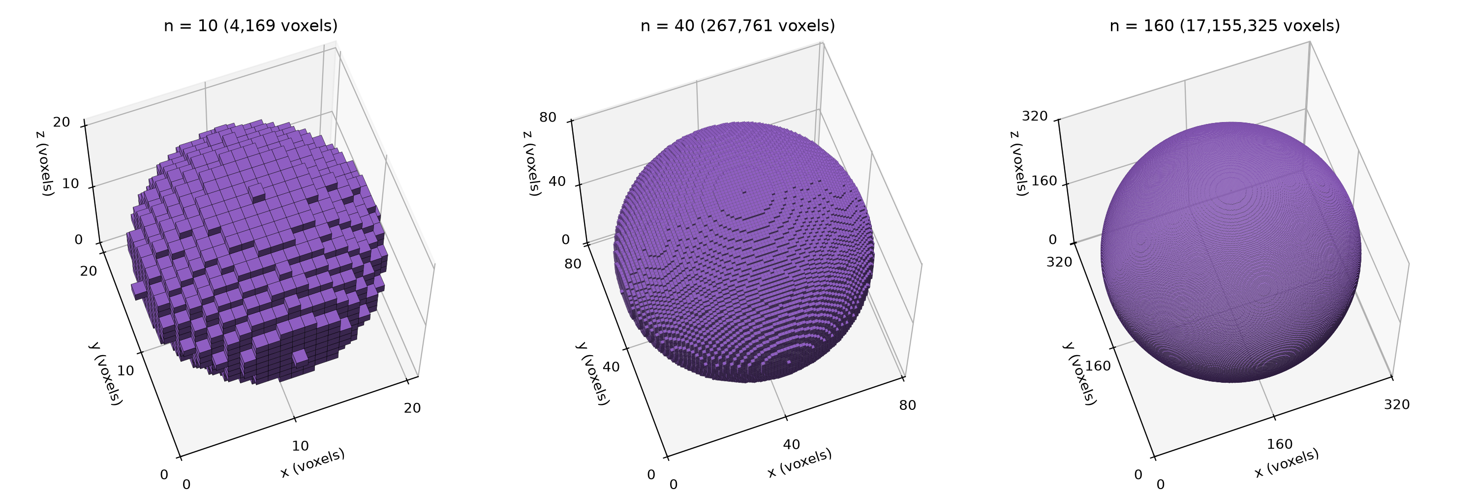
unit_sphere_meshes.py.Marching Cubes
Marching cubes turns a grid of values into a triangulated surface at one
level of those values. The command automesh mesh tri --cubes marching runs
the method of Lewiner et al.1 For each segmentation, automesh
- pads the segmentation by one voxel of zeros, so the surface closes,
- runs marching cubes at level
0.5, halfway between outside (0) and inside (1), - winds every triangle outward, and
- scales and translates the vertices to a unit sphere (see Transform).
The command below meshes the segmentation. The scale is and the translation is in each direction.
automesh mesh tri -i unit_sphere_n010.npy -o unit_sphere_mc_n010.stl --cubes marching \
    --xscale 0.1 --yscale 0.1 --zscale 0.1 \
    --xtranslate -1.05 --ytranslate -1.05 --ztranslate -1.05
The loop below makes the surface for each of the five segmentations.
for n in 10 20 40 80 160; do
  s=$(python3 -c "print(1/$n)")
  t=$(python3 -c "print(-($n + 0.5)/$n)")
  automesh mesh tri -i unit_sphere_n$(printf %03d $n).npy \
    -o unit_sphere_mc_n$(printf %03d $n).stl --cubes marching \
    --xscale $s --yscale $s --zscale $s \
    --xtranslate $t --ytranslate $t --ztranslate $t
done
The surfaces below have the following counts. , , and count the vertices, edges, and faces. The volume is the signed volume that the faces enclose. The error compares that volume with the exact volume .
| volume | error | ||||
|---|---|---|---|---|---|
| 10 | 1,902 | 5,700 | 3,800 | 4.1478 | −0.98% |
| 20 | 7,542 | 22,620 | 15,080 | 4.1699 | −0.45% |
| 40 | 30,150 | 90,444 | 60,296 | 4.1825 | −0.15% |
| 80 | 120,486 | 361,452 | 240,968 | 4.1865 | −0.06% |
| 160 | 482,286 | 1,446,852 | 964,568 | 4.1882 | −0.01% |
The volume created from marching cubes underestimates the true value at every in the table. The surface also encloses less volume than the voxels it came from. This pattern holds at every from 4 to 160. Marching cubes cuts each corner of the voxel staircase with a flat triangle, and every cut removes a small volume.
Five integrity checks run on the five surfaces. All five surfaces give the same result on every check.
- Closed. No edge is open. An open edge belongs to one face only.
- Manifold. No edge is pinched. A pinched edge belongs to more than two faces.
- Oriented. No two faces traverse the same edge in the same direction.
- Connected. The surface is one piece.
- Euler characteristic. .
For a closed, connected, orientable surface, , where is the genus, the number of handles. Here , so , and each surface is topologically a sphere.
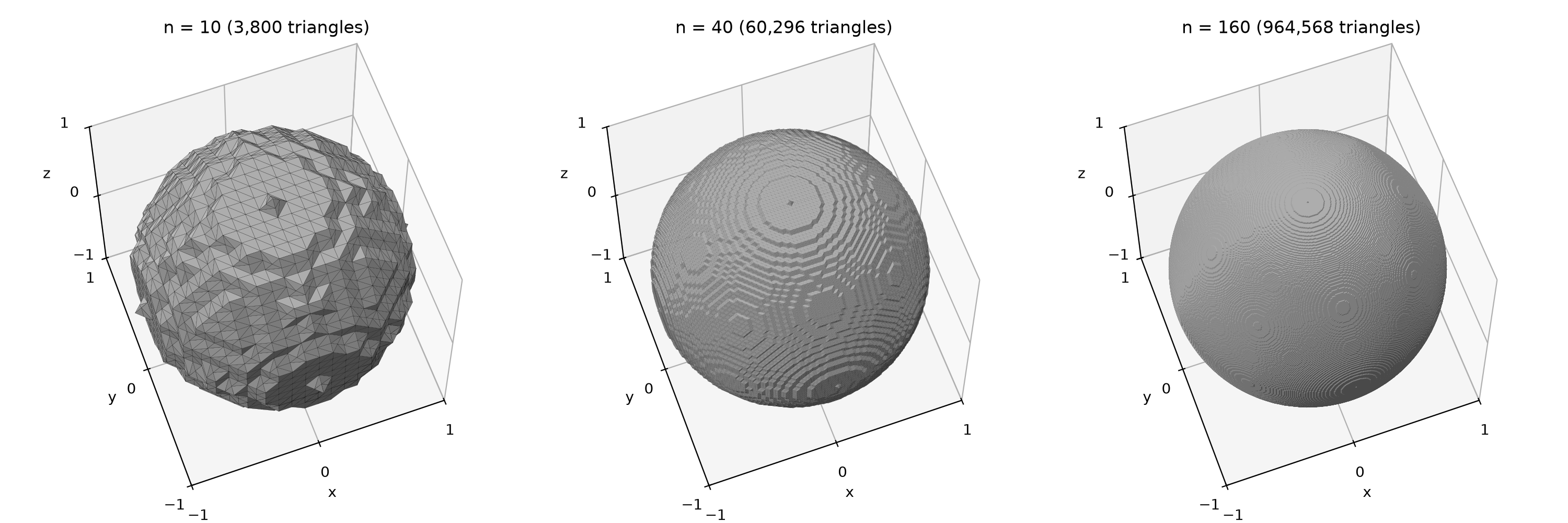
unit_sphere_meshes.py.Convergence
The script
unit_sphere_convergence.py computes both
volumes at every from 4 to 160, 157 values in all. It runs
automesh mesh tri --cubes marching once per .
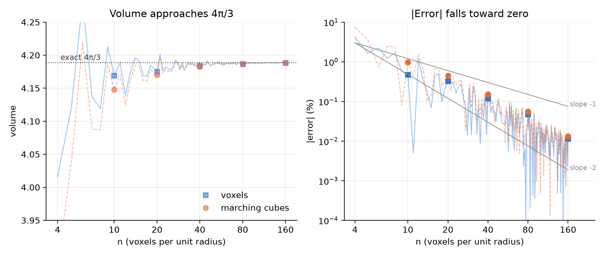
Both volumes settle onto , but neither settles smoothly. The voxel error changes sign 46 times, and 25 of the 157 voxel volumes exceed . The marching cubes error changes sign 24 times, and 12 of its volumes exceed . The five values in the tables just happened to fall short.
Under the oscillation, both errors fall toward zero. A least-squares fit of against gives a slope of −1.71 for the voxels and −1.76 for marching cubes. Both lie between the two guides. The marching cubes volume stays below the voxel volume at all 157 values.
Why Lewiner?
Lorensen and Cline introduced marching cubes in 1987.2 Their method visits each cube of eight neighboring samples. It classifies each corner as inside or outside, which gives 256 cases. Symmetry reduces those to 15 base cases, and each base case has one fixed triangulation.
Some cases are ambiguous. On a face with two inside corners on one diagonal and two outside corners on the other, the corners alone cannot say whether the inside corners connect across the face. An interior ambiguity arises the same way inside a cube. A fixed table picks one answer without looking at the data. Neighboring cubes can then disagree, and the surface can take the wrong topology.
Chernyaev extended the table to 33 cases.3 His table
resolves each ambiguity with the trilinear interpolant of the eight corner
values, the smooth function the samples define inside the cube. Lewiner
et al. gave an efficient and complete implementation of that
table.1 automesh uses the Lewiner method.
The Lewiner method is better than the original table because neighboring cubes always agree. Each ambiguity is resolved from the data, so two cubes that share a face choose the same connection across it. The surface then has the topology of the interpolant's level set.
The sphere reaches no ambiguous case, so the Lewiner method has nothing to resolve here, and no edge of the surface is pinched at any . On data that do reach such cases, the original table can return a surface of different topology. Newman and Yi illustrate each ambiguous case and survey the methods that resolve them.4
A binary mask needs one further caution. On a mask of 0 and 1, the level 0.5 is
exactly the saddle value of an ambiguous face. At that tie, the Lewiner method
can pinch an edge between four faces. automesh uses the level 0.5. The
sphere is a special case that never reaches the tie.
Transform
Marching cubes returns vertices in voxel units. Voxel spans , so the voxel at index spans . That voxel is the center of the sphere, so the center sits at its midpoint, . Two operations map the surface to a unit sphere at the origin.
- Scale by , which makes the radius 1.
- Translate by , which moves the center to the origin.
The --xscale and --xtranslate options of automesh scale first and
translate second, in that order. The translation must use . A
translation of treats the center as the upper face of voxel ,
at . It leaves the surface off center by in each direction.
The vertex radii show how close the surface comes to the unit sphere. The coefficient of variation, CoV , measures how much the radii spread. A perfect sphere has CoV .
| min | max | mean | CoV | |
|---|---|---|---|---|
| 10 | 0.9552 | 1.0500 | 0.9993 | 2.15% |
| 20 | 0.9763 | 1.0250 | 0.9991 | 1.01% |
| 40 | 0.9878 | 1.0125 | 0.9996 | 0.51% |
| 80 | 0.9938 | 1.0063 | 0.9999 | 0.26% |
| 160 | 0.9969 | 1.0031 | 1.0000 | 0.13% |
The mean radius stays within 0.1% of 1 at every , so a scale of leaves no bias. The largest radius is always , at the six poles. There a vertex sits halfway between the last inside voxel, at radius , and the first outside voxel, at radius .
The CoV halves each time doubles, so the spread of the radii falls as . That is first order, slower than the volume error in Convergence. The volume averages over the whole surface, and the staircase steps partly cancel in that average. The radius spread sees every step.
Surface Comparison
Hausdorff Distance
The Hausdorff distance between two surfaces is the farthest that any point of either one lies from the other. For a surface and the unit sphere ,
The script unit_sphere_comparison.py computes the
first term exactly. A point lies from
the unit sphere. Over a triangle, is convex. Its largest value sits at
a vertex, and its smallest sits at the point of the triangle closest to the
origin.5 The largest over all triangles gives the
outward distance. The largest gives the inward distance.
The second term needs no computation. Each surface is closed and encloses the origin. The ray from the origin through a sphere point therefore crosses at some point . Then . The second term never exceeds the first, so the Hausdorff distance is the larger of the outward and inward distances.
uv run --with numpy unit_sphere_comparison.py
| outward | inward | ||||
|---|---|---|---|---|---|
| 10 | 3,800 | 0.05000 | 0.04737 | 0.05000 | 0.500 |
| 20 | 15,080 | 0.02500 | 0.02436 | 0.02500 | 0.500 |
| 40 | 60,296 | 0.01250 | 0.01234 | 0.01250 | 0.500 |
| 80 | 240,968 | 0.00625 | 0.00621 | 0.00625 | 0.500 |
| 160 | 964,568 | 0.00312 | 0.00312 | 0.00312 | 0.500 |
The Hausdorff distance is exactly at every , half a voxel. The outward distance sets it, at the six poles (see Transform). The inward distance approaches it from below. The Hausdorff distance falls as , first order, like the radius CoV. The triangle count grows as , so in terms of triangles the distance falls only as .
Surface Area
The volume converges, as the Convergence section shows. The
surface area does not converge. The script
unit_sphere_comparison.py adds up the areas of
the marching cubes triangles. The error compares that area with the exact
area .
| area | error | |
|---|---|---|
| 10 | 13.7204 | +9.18% |
| 20 | 13.6324 | +8.48% |
| 40 | 13.6566 | +8.68% |
| 80 | 13.6608 | +8.71% |
| 160 | 13.6673 | +8.76% |
The voxel staircase itself would overstate the area by 50% at any . Marching cubes cuts the voxel staircase corners, which removes most of that excess. Howver, the surface area still settles near 8.8% too large.
Smaller voxels make smaller steps, but the triangles keep the same few orientations relative to the true surface. So the Hausdorff distance falls to zero while the area error does not. A surface can come arbitrarily close to the sphere and still have the wrong area.
Triangle Quality
The script unit_sphere_comparison.py also runs
automesh metrics on each surface. The
Triangular Metrics page defines its
measures.
A binary mask puts every vertex at the midpoint of a cube edge. So marching cubes can make only a few triangle shapes. Grouped by maximum edge ratio and minimum scaled Jacobian, the triangular surfaces created by marching cubes produce exactly five shapes. The table gives the fraction of triangles of each shape.
| shape | angles | edge ratio | scaled Jacobian | |||||
|---|---|---|---|---|---|---|---|---|
| equilateral | 60°, 60°, 60° | 1.000 | 1.000 | 14.74% | 14.80% | 14.30% | 13.99% | 13.98% |
| right isosceles | 45°, 45°, 90° | 1.414 | 0.816 | 24.63% | 25.15% | 25.04% | 24.92% | 24.85% |
| right | 35.26°, 54.74°, 90° | 1.732 | 0.667 | 31.58% | 30.56% | 32.08% | 33.13% | 33.20% |
| obtuse isosceles | 30°, 30°, 120° | 1.732 | 0.577 | 14.53% | 14.75% | 14.29% | 13.98% | 13.98% |
| 30-60-90 | 30°, 60°, 90° | 2.000 | 0.577 | 14.53% | 14.75% | 14.29% | 13.98% | 13.98% |
Refinement does not change the quality. The same five shapes appear at every , in nearly the same proportions. More than a quarter of the triangles have the worst scaled Jacobian, , with a smallest angle of 30°. No triangle is worse.
Smaller voxels shrink the triangles but never reshape them. A histogram of any measure would show only these five spikes, so the table is shown instead of a histogram.
Mesh
Sculpt
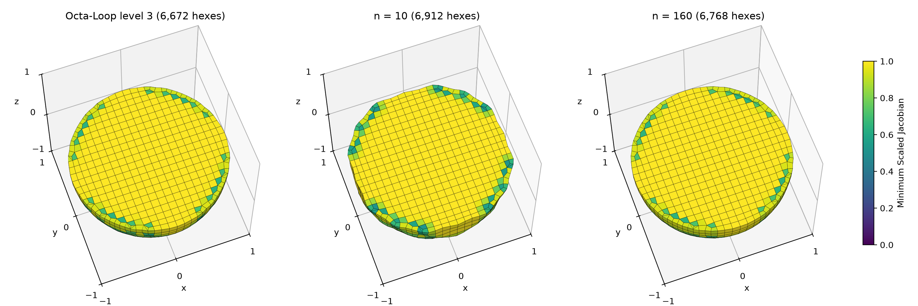
The Subdivision page meshes its Octa-Loop spheres with Sculpt. At levels 3 to 7, it reports a grid of 26×26×26 cells, 7,731 nodes, and 6,672 elements. Here Sculpt meshes the marching cubes surfaces on the same grid.
The Subdivision baseline runs Sculpt through Cubit's sculpt parallel
command, which chooses the grid itself. For Octa-Loop level 3, Cubit places 26
cells in each direction across a box of , a cell size of about
0.0954. Standalone Sculpt with those options reproduces the baseline exactly,
at 7,731 nodes and 6,672 elements. The same options mesh each marching cubes
surface.
B=1.240409
GRID="-x 26 -y 26 -z 26 -t -$B -u -$B -v -$B -q $B -r $B -s $B -SS 2"
# octa_loop03.stl downloads from the Refinement table of the Subdivision page
sculpt -j 1 -stl octa_loop03.stl $GRID -e unit_sphere_sculpt_octa03
for n in 010 020 040 080 160; do
  sculpt -j 1 -stl unit_sphere_mc_n$n.stl $GRID -e unit_sphere_sculpt_n$n
done
Left to choose its own grid, Cubit sizes the cells to the small marching cubes facets. For it picks 73×73×73 cells and makes 180,201 elements. Fixing the grid keeps the meshes comparable with the baseline.
The quality is the minimum scaled Jacobian, as Sculpt reports it.
| input | nodes | elements | minimum quality | mean quality |
|---|---|---|---|---|
| Octa-Loop level 3 (baseline) | 7,731 | 6,672 | 0.343 | 0.888 |
| marching cubes, | 8,007 | 6,912 | 0.388 | 0.885 |
| marching cubes, | 7,827 | 6,768 | 0.404 | 0.900 |
| marching cubes, | 7,827 | 6,768 | 0.420 | 0.902 |
| marching cubes, | 7,827 | 6,768 | 0.401 | 0.901 |
| marching cubes, | 7,827 | 6,768 | 0.427 | 0.901 |
From on, every surface gives the same 7,827 nodes and 6,768 elements, 96 more of each than the baseline, or about 1.4%. The worst element is better than the baseline's at every .
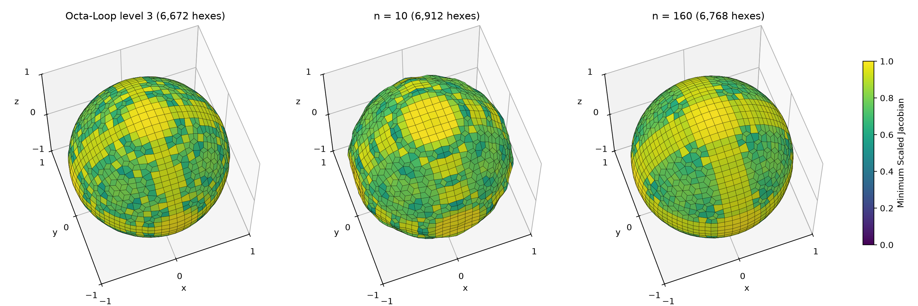
unit_sphere_meshes.py.The difference between the middle and right panels comes from the size of a voxel step against the size of a Sculpt cell, about 0.095.
- At , a voxel is 0.1 wide, so each step is about as large as a cell. The mesh boundary follows the steps, and the sphere looks lumpy.
- At , a voxel is 0.00625 wide, so a cell spans about 15 voxels. The steps are far smaller than the elements, and the mesh looks like the baseline.
- From on, a cell spans about two voxels or more, and the mesh stops changing.
unit_sphere_meshes.py.The run used Sculpt 16.08, from Cubit 16.08. The files unit_sphere_sculpt_*.e.1.0
are Sculpt outputs, and the repository does not contain them. The scripts of
this page read them from this directory, so regenerating the Sculpt figures and
table requires running the Sculpt commands above. automesh reads Sculpt's Exodus
files directly, and automesh metrics gives the same minimum (0.343) and mean
(0.888) as Sculpt for the baseline mesh.
automesh
automesh mesh hex meshes the marching cubes surface in two ways.
The uniform mesh uses the Sculpt cell size, , so its lattice matches the Sculpt grid. The adaptive mesh uses the
defaults.
automesh mesh hex -i unit_sphere_mc_n010.stl -o uniform.inp \
  -u 0.095416 --metrics uniform.csv
automesh mesh hex -i unit_sphere_mc_n010.stl -o adaptive.inp \
  --metrics adaptive.csv
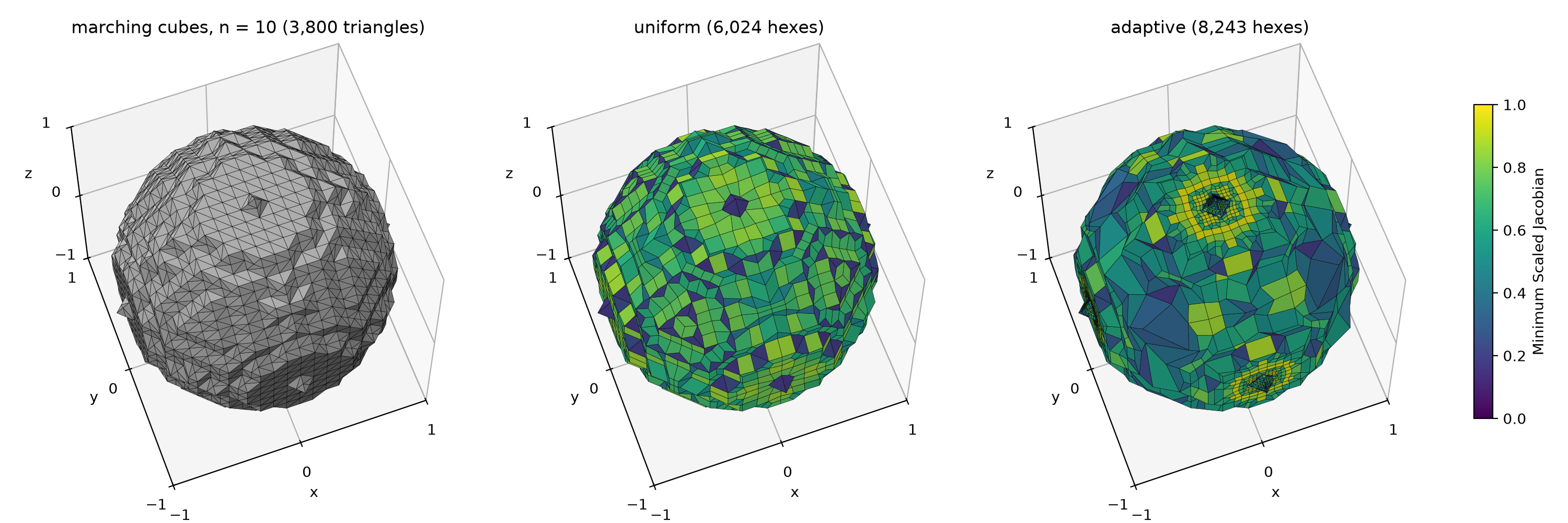
unit_sphere_mc_n010.stl, (center) automesh uniform, (right) automesh adaptive.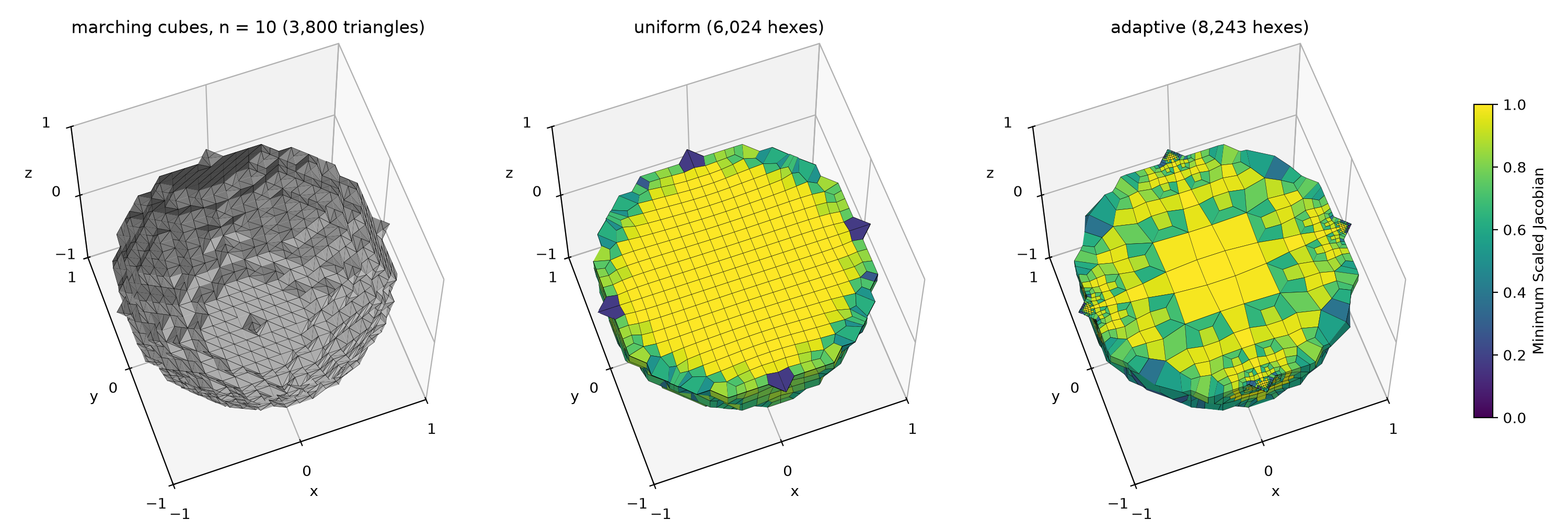
automesh uniform and adaptive, both without prior smoothing of the marching cubes surface.Taubin Smoothing
Taubin smoothing rounds the voxel steps of the surface. This section measures how the number of smoothing iterations changes the Minimum Scaled Jacobian of the uniform and adaptive meshes.
automesh smooth applies Taubin smoothing with its defaults. The pass band is
0.1 and the scale is , which gives . Each
iteration is one Laplacian step. Odd-numbered iterations shrink the surface
with . Even-numbered iterations inflate it with . The sweep runs
every integer from 0 to 100 iterations, every tenth from 110 to 300, and every
fiftieth from 350 to 1,000. Each smoothed surface gets a uniform mesh with the
Sculpt cell size and an adaptive mesh with the defaults.
automesh smooth -i unit_sphere_mc_n010.stl -o smooth.stl --iterations 260
automesh mesh hex -i smooth.stl -o uniform.inp -u 0.095416 --metrics uniform.csv
automesh mesh hex -i smooth.stl -o adaptive.inp --metrics adaptive.csv
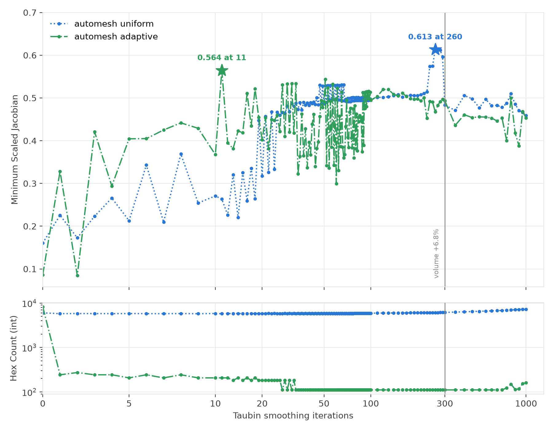
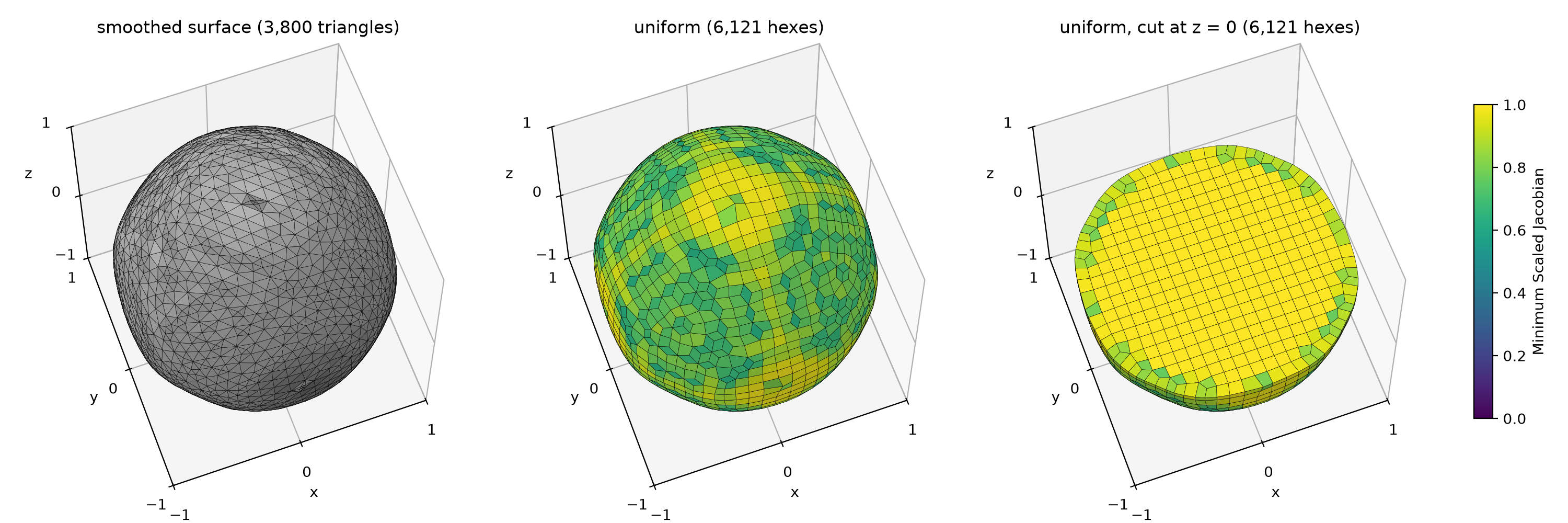
automesh uniform and adaptive meshes of the surface, against the number of Taubin smoothing iterations. Stars mark the peak of each series up to 300 iterations. Each peak is also the highest value of the whole sweep. The vertical line at 300 iterations marks a surface volume 6.8% above the sphere's. The x-axis is linear to 10 iterations and logarithmic beyond.Uniform. The minimum rises with scatter from 0.161 at 0 iterations to 0.613 at 260 iterations. The mean rises from 0.827 to 0.901. Up to 300 iterations the hex count stays between 5,747 and 6,150, against 6,024 without smoothing. The peak is a plateau: 0.613, 0.612, and 0.612 at 260, 270, and 280 iterations, against 0.574 and 0.575 at 240 and 250. The minimum then falls to 0.483 at 300 iterations and scatters between 0.459 and 0.510 up to 1,000.
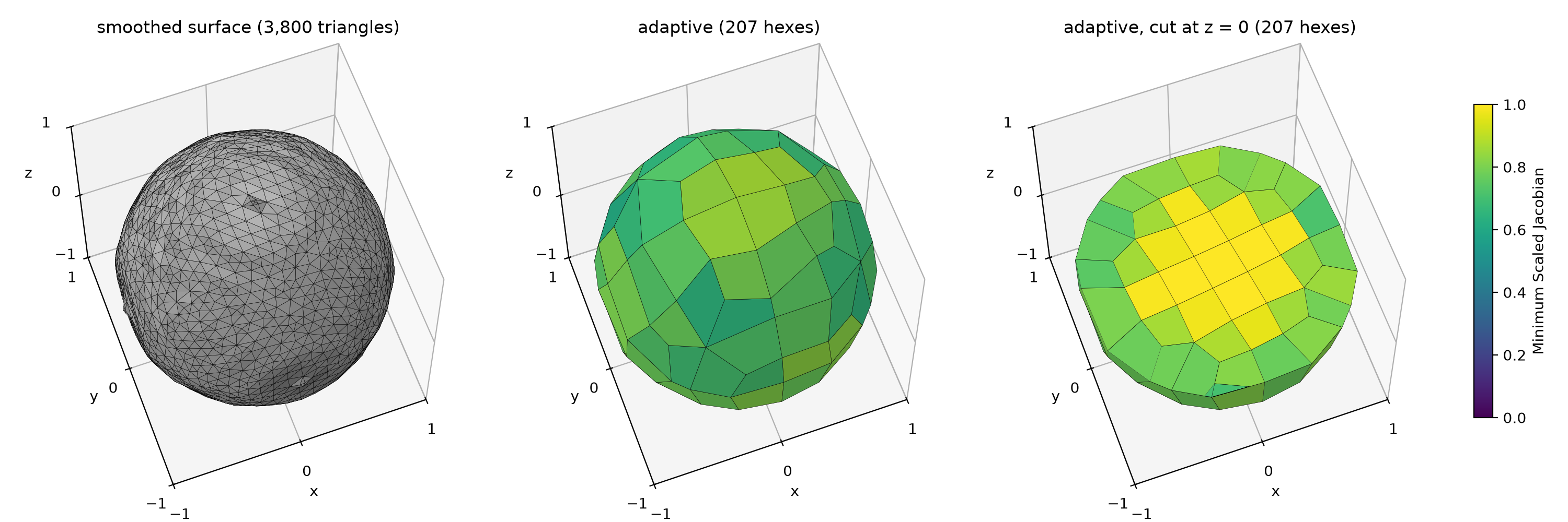
Adaptive. The hex count falls from 8,243 at 0 iterations to 243 at 1 iteration. From 34 to 700 iterations it stays at 111 hexes. The minimum peaks at 0.564 at 11 iterations, on 207 hexes. The peak is a spike, not a plateau. The minimum is 0.367 at 10 iterations and 0.395 at 12. The next highest minimum is 0.544 at 51 iterations, on 111 hexes. The 111-hex meshes start at 0.323 at 34 iterations and scatter between 0.299 and 0.544 up to 700.
Surface drift. The defaults inflate this surface, because exceeds . The mean vertex radius grows from 0.9992 at 0 iterations to 1.0207 at 260 and 1.0862 at 1,000. The enclosed volume is 4.126 at 11 iterations, 1.5% below . It is 4.428 at 260 iterations, 5.7% above, and 5.322 at 1,000, 27.1% above. The peak search therefore stops at 300 iterations.
Odd and even counts. An odd count ends on a shrink step and an even count on an inflate step, so neighboring counts give different surfaces. The enclosed volume is 4.115 at 1 iteration and 4.149 at 2. The adaptive minimum is 0.328 at 1 iteration and 0.085 at 2. The uniform minimum is 0.223 at 3 iterations and 0.266 at 4.
None of the 270 meshes has an inverted hex.
Quality After Smoothing
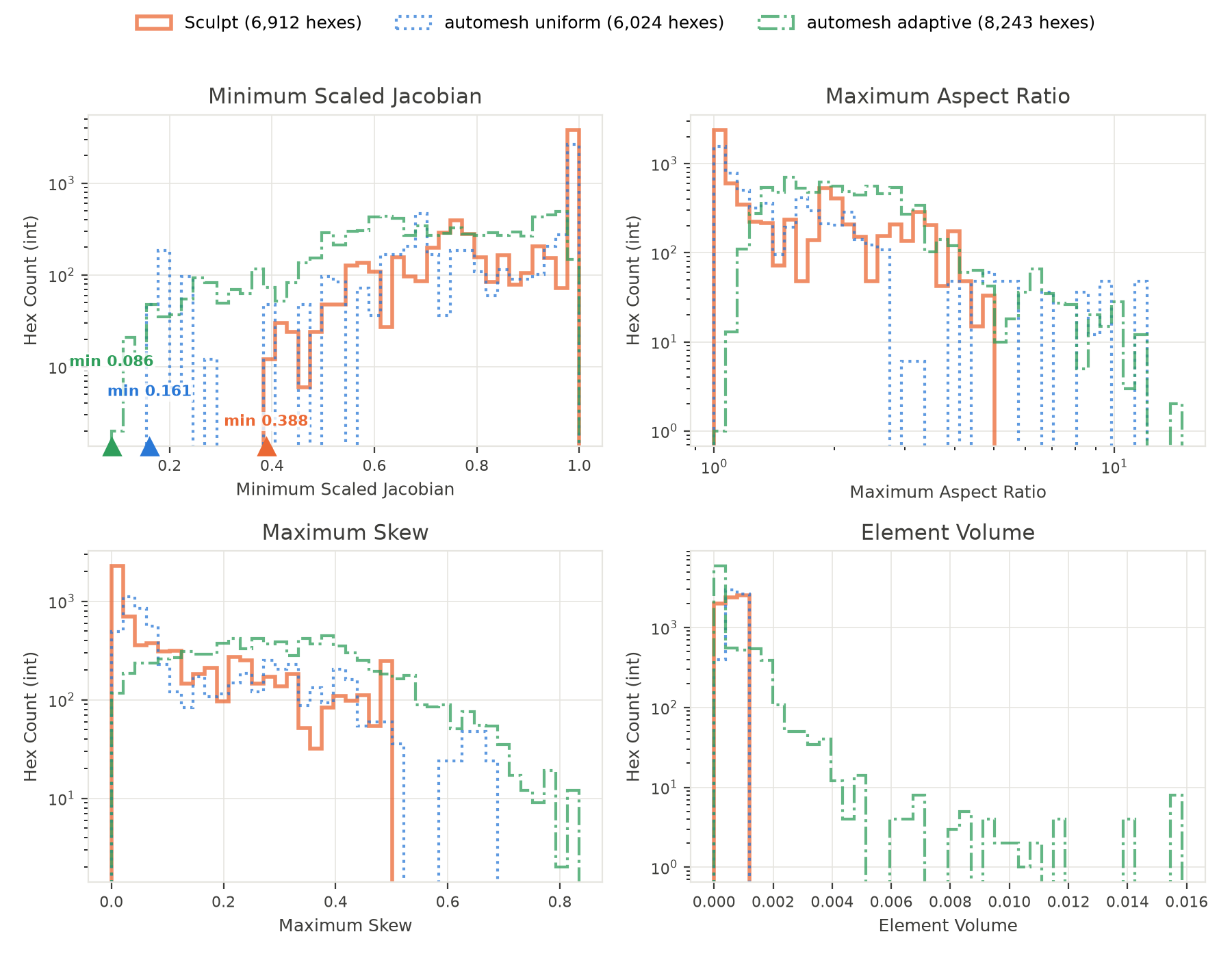
The figure below compares the two best meshes of the sweep with the same meshes before smoothing and with the Sculpt baseline. The uniform mesh comes from the surface smoothed 260 times, with a minimum of 0.613. The adaptive mesh comes from the surface smoothed 11 times, with a minimum of 0.564. Without smoothing, the minima are 0.161 and 0.086. The Sculpt minimum is 0.388.
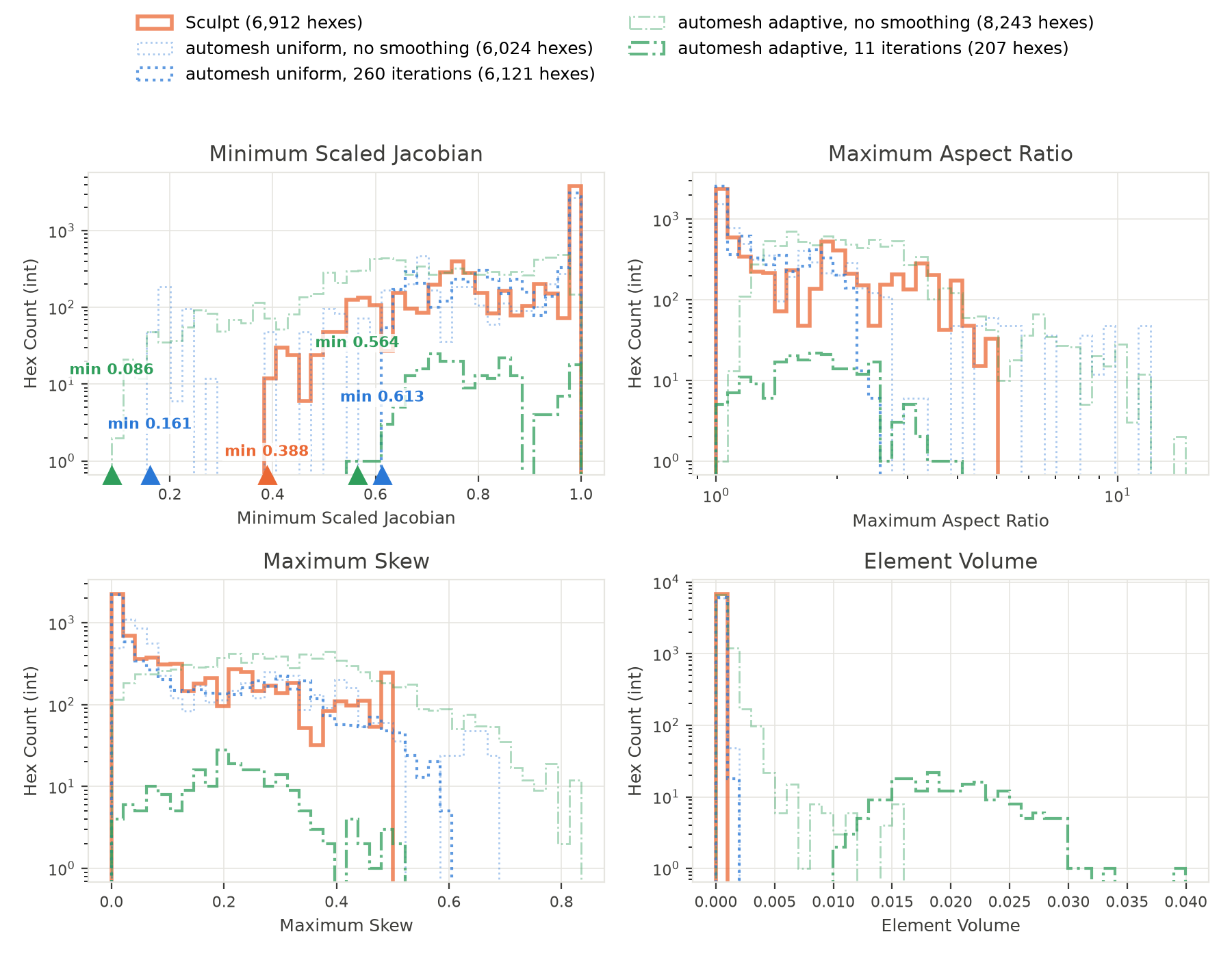
automesh uniform mesh after 260 Taubin smoothing iterations and the adaptive mesh after 11, the best Minimum Scaled Jacobian of each, against the same meshes without smoothing (faint lines) and the Sculpt mesh for . The figure is produced by unit_sphere_smooth.py.| input | nodes | elements | minimum quality | mean quality |
|---|---|---|---|---|
| Octa-Loop level 3 (baseline) | 7,731 | 6,672 | 0.343 | 0.888 |
| marching cubes, | 8,007 | 6,912 | 0.388 | 0.885 |
| automesh uniform, before smoothing | 7,035 | 6,024 | 0.161 | 0.827 |
| automesh adaptive, before smoothing | 10,016 | 8,243 | 0.086 | 0.694 |
| automesh uniform, best result with smoothing (260 iterations) | 7,120 | 6,121 | 0.613 | 0.901 |
| automesh adaptive, best result with smoothing (11 iterations) | 288 | 207 | 0.564 | 0.793 |
The quality is the minimum scaled Jacobian, as in the Sculpt table. The first two rows, the Sculpt meshes of the Sculpt section, are the reference. Smoothing raises the uniform minimum from 0.161 to 0.613 and the adaptive minimum from 0.086 to 0.564. Of the two best meshes, the uniform mesh has the higher minimum, by 0.049, and the higher mean, by 0.108.
The adaptive mesh has 207 hexes, 3.4% of the uniform count, so its histograms sit about a factor of 30 lower. Compare the shapes of the curves, not their heights.
The two minima differ in how robust they are. The uniform value belongs to a plateau: 0.613, 0.612, and 0.612 at 260, 270, and 280 iterations. The adaptive value belongs to a spike: 0.367 at 10 iterations, 0.564 at 11, and 0.395 at 12. A small change in the iteration count would lose the adaptive result.
Control Study
automesh mesh hex's adaptive octree combines two refinement signals:
- curvature-driven sizing, gated by a chord-error tolerance
(
--tolerance, disabled by default), and - local-thickness sizing, from the shape diameter function of Shapira, Shamir, and Cohen-Or.6
No script on this page passes --tolerance, so curvature-driven sizing never
activates here. Local thickness alone (not curvature) sets the octree's
refinement target.
Taubin smoothing raised the Minimum Scaled Jacobian of the marching cubes
meshes, from 0.161 to 0.613 for the uniform mesh and from 0.086 to 0.564 for the
adaptive mesh. The control study asks whether a surface that is already smooth
does better than that. The control is Octa-Loop level 4, a Loop subdivision of
an octahedron from the Subdivision
page. Its file, octa_loop04.stl, downloads from the Refinement table. The
surface is closed, has 2,048 triangles, and its 1,026 vertices lie within 0.3% of
the unit sphere.
Level 4 is the level whose triangle count is closest to that of the smoothed surface. Smoothing moves the vertices and leaves the count at 3,800. Level 3 has 512 triangles, level 4 has 2,048, and level 5 has 8,192. The mean triangle edge points the same way: 0.118 for level 4 against 0.092 for the smoothed surface, and about 0.059 for level 5, since each level halves the edge.
automesh mesh hex -i octa_loop04.stl -o octa_uniform.inp \
  -u 0.095416 --metrics octa_uniform.csv
automesh mesh hex -i octa_loop04.stl -o octa_adaptive.inp \
  --metrics octa_adaptive.csv
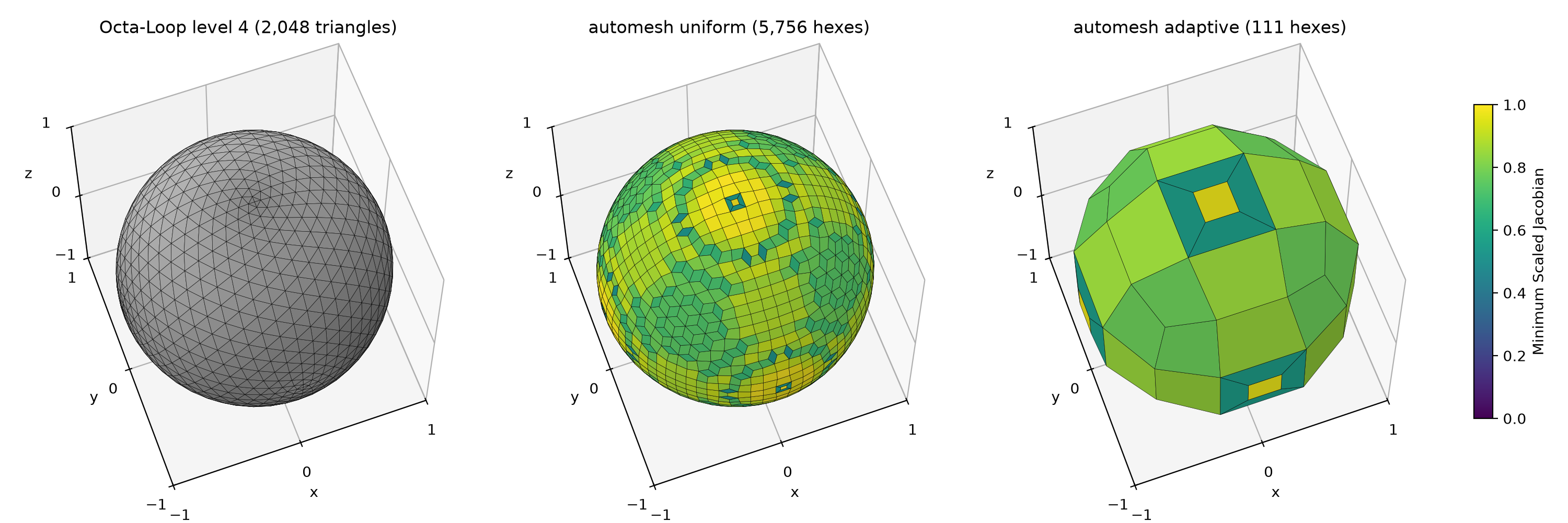
octa_loop04.stl (2,048 triangles), (center) automesh uniform (5,756 hexes), (right) automesh adaptive (111 hexes).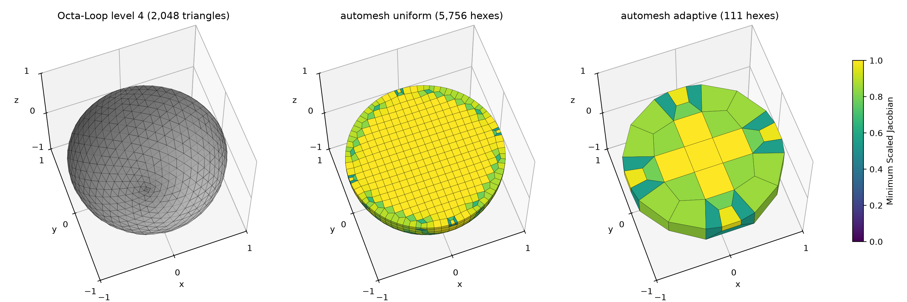
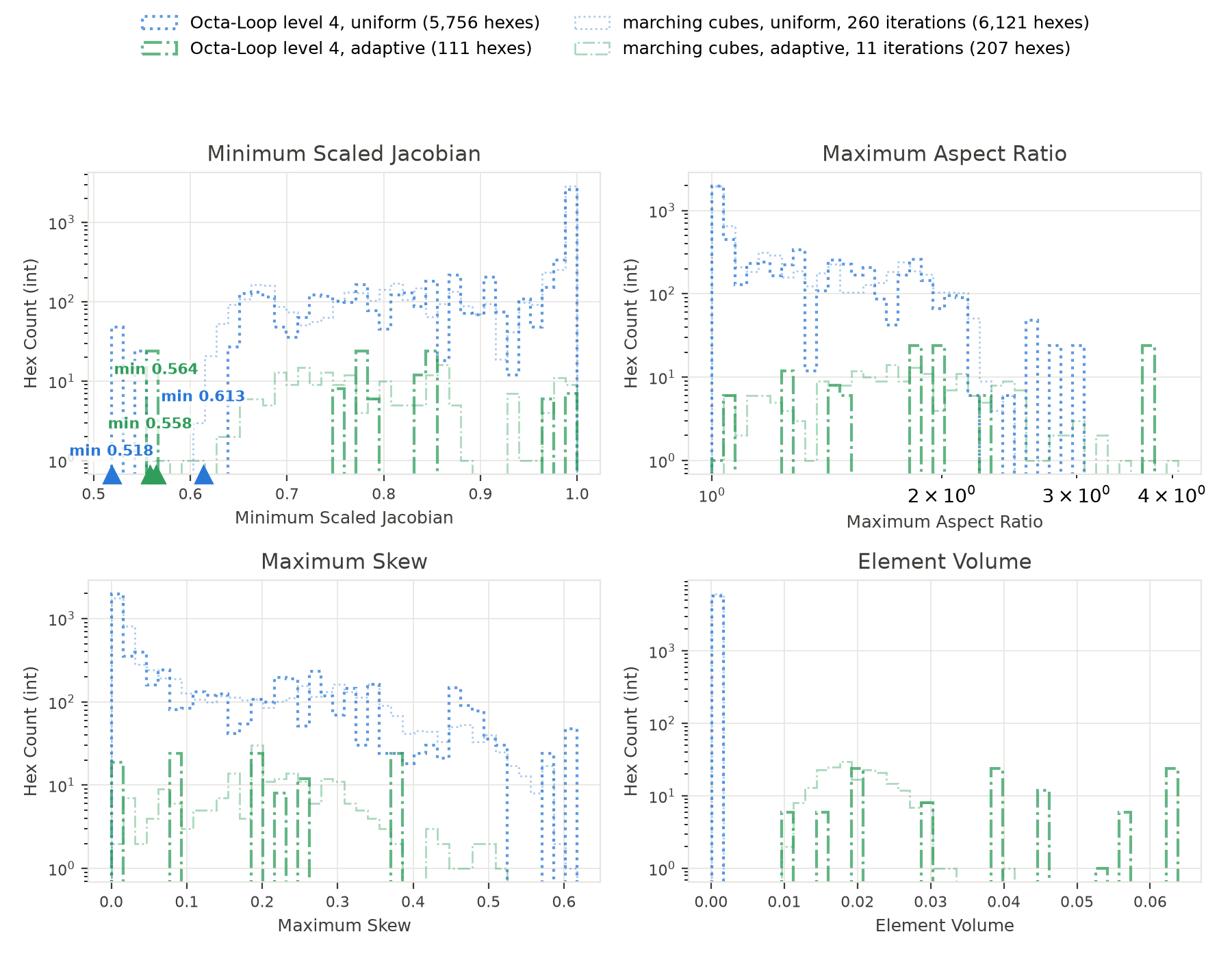
automesh uniform and adaptive meshes of Octa-Loop level 4, against the best Taubin-smoothed marching cubes meshes of the previous section (faint lines). The figure is produced by unit_sphere_control.py.| input | nodes | elements | minimum quality | mean quality |
|---|---|---|---|---|
| marching cubes, uniform, best result with smoothing (260 iterations) | 7,120 | 6,121 | 0.613 | 0.901 |
| marching cubes, adaptive, best result with smoothing (11 iterations) | 288 | 207 | 0.564 | 0.793 |
| Octa-Loop level 4, uniform | 6,737 | 5,756 | 0.518 | 0.903 |
| Octa-Loop level 4, adaptive | 168 | 111 | 0.558 | 0.775 |
The smooth surface does not beat the best smoothed surface. The uniform mesh of Octa-Loop level 4 has a minimum of 0.518, which is 0.095 below the best smoothed marching cubes mesh, and a mean of 0.903, which is 0.002 above it. The adaptive mesh has a minimum of 0.558, 0.006 below, and a mean of 0.775, 0.018 below. The adaptive mesh has 111 hexes, against 207.
The comparison favors the smoothed surface, because its result is the maximum of 135 iteration counts and the Octa-Loop result is one run. Only 17 of the 135 counts give a uniform minimum above 0.518. Only 1 gives an adaptive minimum above 0.558, the best one itself. From 100 iterations on, the median minimum is 0.503 for the uniform mesh and 0.492 for the adaptive mesh, and the Octa-Loop values are above both. Against the unsmoothed marching cubes meshes, the Octa-Loop minima are 0.518 against 0.161 for the uniform mesh and 0.558 against 0.086 for the adaptive mesh.
A smooth input surface reaches, in one run and with no search over iteration counts, a minimum within 0.006 of the best smoothed adaptive result, and 0.095 below the best smoothed uniform result. None of the four meshes has an inverted hex.
-
Thomas Lewiner, Hélio Lopes, Antônio Wilson Vieira, and Geovan Tavares. "Efficient implementation of Marching Cubes' cases with topological guarantees." Journal of Graphics Tools 8(2) (2003) 1–15. https://doi.org/10.1080/10867651.2003.10487582 ↩ ↩2
-
William E. Lorensen and Harvey E. Cline. "Marching cubes: A high resolution 3D surface construction algorithm." ACM SIGGRAPH Computer Graphics 21(4) (1987) 163–169. https://doi.org/10.1145/37402.37422 ↩
-
Evgeni V. Chernyaev. Marching Cubes 33: Construction of topologically correct isosurfaces. Technical Report CN/95-17, CERN, 1995. ↩
-
Timothy S. Newman and Hong Yi. "A survey of the marching cubes algorithm." Computers & Graphics 30(5) (2006) 854–879. https://doi.org/10.1016/j.cag.2006.07.021 ↩
-
Christer Ericson. Real-Time Collision Detection. Morgan Kaufmann, 2005. Section 5.1.5, the closest point on a triangle to a point. ↩
-
Lior Shapira, Ariel Shamir, and Daniel Cohen-Or. "Consistent mesh partitioning and skeletonisation using the shape diameter function." The Visual Computer 24 (2008) 249–259. https://doi.org/10.1007/s00371-007-0197-5 ↩