Introduction
automesh is an open-source Rust software program that uses a segmentation,
typically generated from a 3D image stack,
or a tessellation (a triangular surface)
to create a finite element mesh.
- The volumetric elements are hexahedral, tetrahedral, hex-dominant, or polyhedral.
- The surface elements are triangular (isosurface).
automesh converts between
segmentation formats (.npy, .spn, .vti)
and
mesh formats (.exo, .inp, .mesh, .off, .stl, .vtu).
automesh can defeature voxel domains,
apply Laplacian and Taubin smoothing, with an optional hierarchical mode,
and output mesh quality metrics.
automesh can also extract a sub-range of voxels from a segmentation,
diff two segmentations to show where they differ, segment a mesh back
into a voxel domain, remesh a triangular surface with uniform or
curvature-adaptive sizing, and partition a mesh into parts written as one
.exo file per part.
Segmentation
Segmentation is the process of categorizing pixels that compose a digital image into a class that represents some subject of interest. For example, in the image below, the image pixels are classified into classes of sky, trees, cat, grass, and cow.
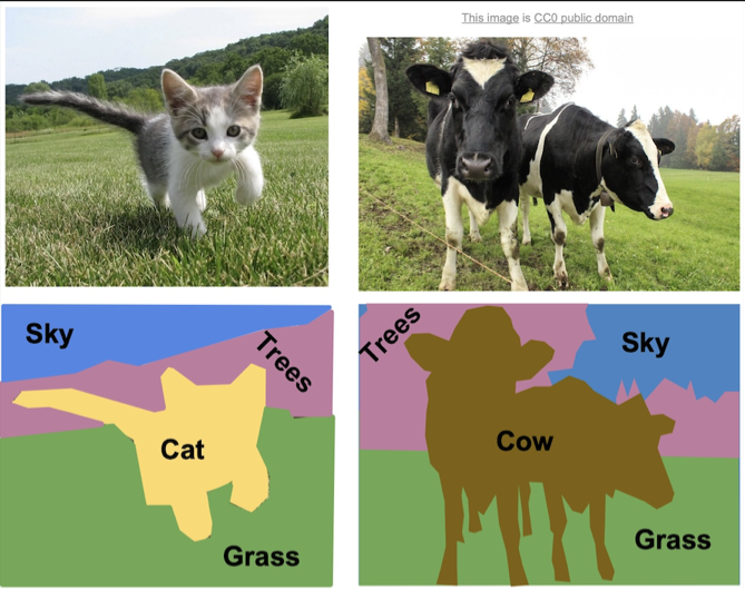
Example of semantic segmentation, from Li et al.1
- Semantic segmentation does not differentiate between objects of the same class.
- Instance segmentation does differentiate between objects of the same class.
These two concepts are shown below:
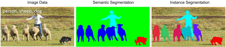
Distinction between semantic segmentation and instance segmentation, from Lin et al.2
Both segmentation types, semantic and instance, can be used with automesh. However, automesh operates on a 3D segmentation, not a 2D segmentation, as present in a digital image. To obtain a 3D segmentation, two or more images are stacked to compose a volume.
The structured volume of a stack of pixels composes a volumetric unit called a voxel. A voxel, in the context of this work, will have the same dimensionality in the x and y dimension as the pixel in the image space, and will have the z dimensionality that is the stack interval distance between each image slice. All pixels are rectangular, and all voxels are cuboid.
The figure below illustrates the concept of stacked images:
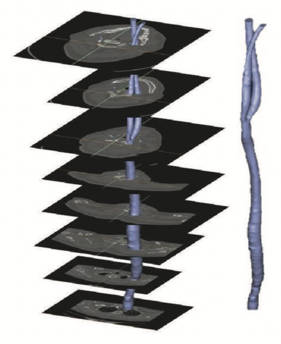
Example of stacking several images to create a 3D representation, from Bit et al.3
The digital image sources are frequently medical images, obtained by CT or MR, though automesh can be used for any subject that can be represented as a stacked segmentation. Anatomical regions are classified into categories. For example, in the image below, ten unique integers have been used to represent
bone, disc, vasculature, airway/sinus, membrane, cerebral spinal fluid, white matter, gray matter, muscle, and skin.
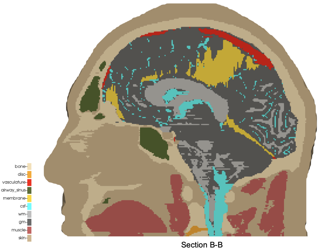
Example of a 3D voxel model, segmented into 10 categories, from Terpsma et al.4
Given a 3D segmentation, for any image slice that composes it, the pixels have been classified
into categories that are designated with unique, non-negative integers.
The range of integer values is limited to 256 = 2^8, since the uint8 data type is specified.
A practical example of a range could be [0, 1, 2, 3, 4]. The integers do not need to be sequential,
so a range of [4, 501, 2, 0, 42] is also valid, but not conventional.
Segmentations are frequently serialized (saved to disc) as either a NumPy (.npy) file
or a SPN (.spn) file.
A SPN file is a text (human-readable) file that contains a single column of non-negative integer values. Each integer value defines a unique category of a segmentation.
Axis order (for example,
x, y, then z; or, z, y, x, etc.) is not implied by the SPN structure;
so additional data is needed to uniquely interpret the pixel tile and voxel
stack order of the data in the SPN file. automesh takes this as the
--nelx, --nely, and --nelz command line arguments.
For subjects that are human anatomy, we use the Patient Coordinate System (PCS), which directs the
x, y, and z axes to the left, posterior, and superior, as shown below:
| Patient Coordinate System: | Left, Posterior, Superior (x, y, z) |
|---|---|
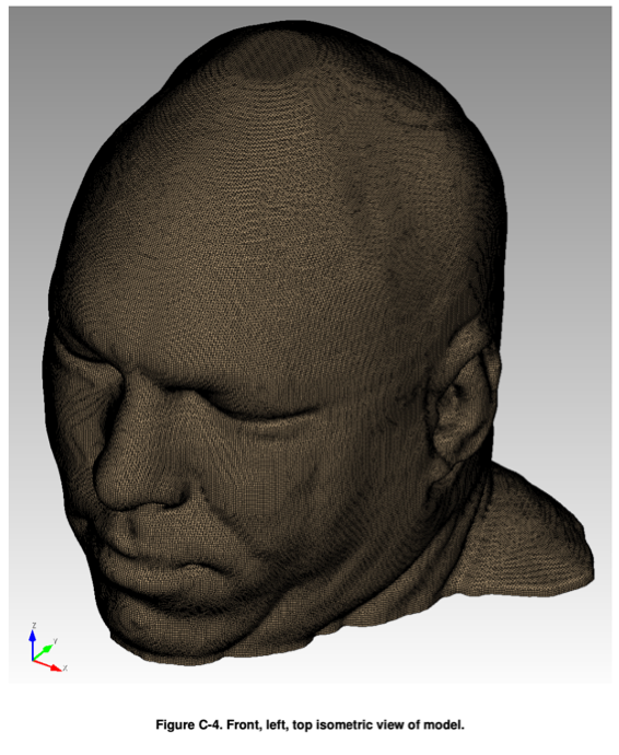 | 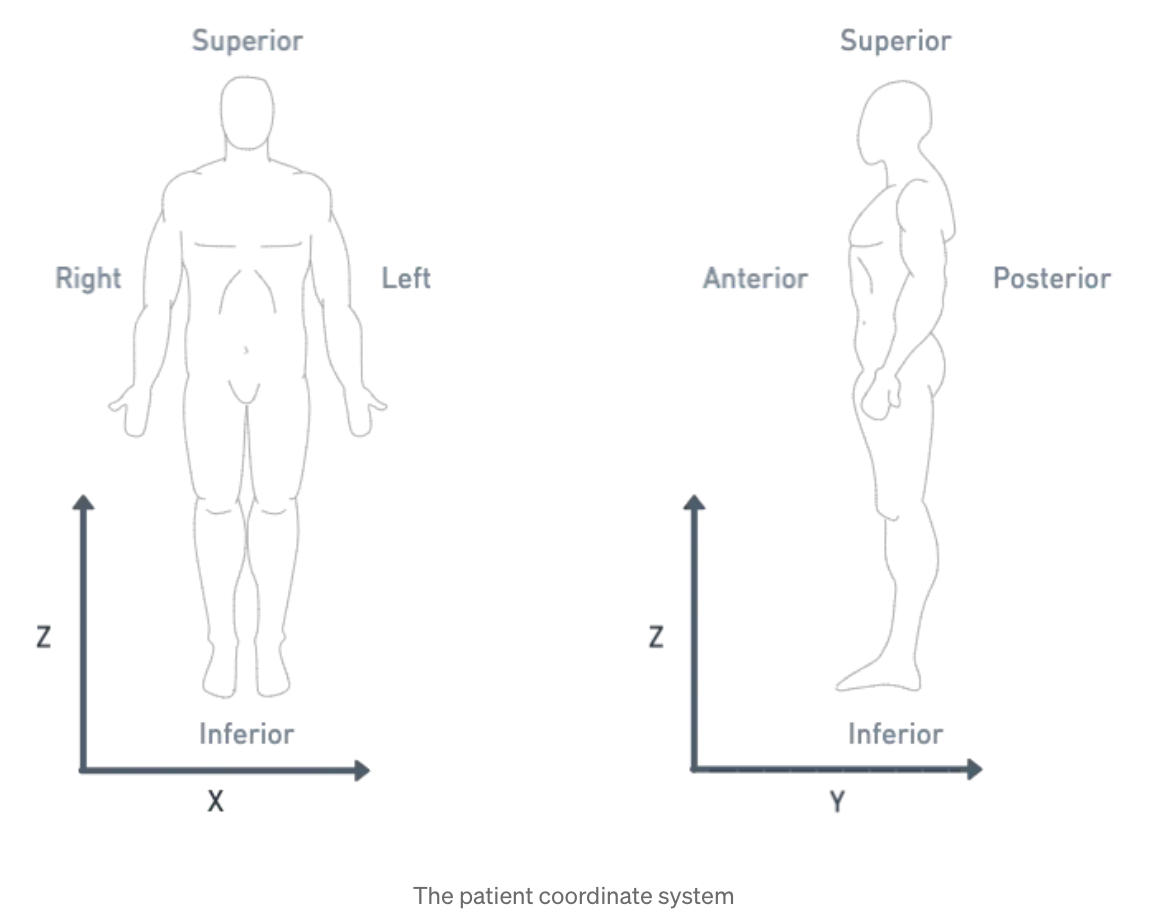 |
Illustration of the patient coordinate system, left figure from Terpsma et al.4 and right figure from Sharma.5
Mesh
automesh writes several mesh formats: .exo, the EXODUS II finite element
data model;6 .inp, the Abaqus input format;7 .mesh,
the Medit format;8 .off, the Object File Format used by
Geomview;9 .stl, the STL format for triangular surfaces in
3D;10 and .vtu, the VTK XML UnstructuredGrid
format.11
References
-
Li FF, Johnson J, Yeung S. Lecture 11: Detection and Segmentation, CS 231n, Stanford University, 2017. link ↩
-
Lin TY, Maire M, Belongie S, Hays J, Perona P, Ramanan D, Dollár P, Zitnick CL. Microsoft coco: Common objects in context. In Computer Vision–ECCV 2014: 13th European Conference, Zurich, Switzerland, September 6-12, 2014, Proceedings, Part V 13 2014 (pp. 740-755). Springer International Publishing. link ↩
-
Bit A, Ghagare D, Rizvanov AA, Chattopadhyay H. Assessment of influences of stenoses in right carotid artery on left carotid artery using wall stress marker. BioMed research international. 2017;2017(1):2935195. link ↩
-
Terpsma RJ, Hovey CB. Blunt impact brain injury using cellular injury criterion. Sandia National Lab. (SNL-NM), Albuquerque, NM (United States); 2020 Oct 1. link ↩ ↩2
-
Sharma S. DICOM Coordinate Systems — 3D DICOM for computer vision engineers, Medium, 2021-12-22. link ↩
-
Schoof LA, Yarberry VR. EXODUS II: a finite element data model. Sandia National Lab. (SNL-NM), Albuquerque, NM (United States); 1994 Sep 1. link ↩
-
Dassault Systèmes Simulia Corp. Abaqus documentation. link ↩
-
Frey PJ. MEDIT: an interactive mesh visualization software. Institut National de Recherche en Informatique et en Automatique (INRIA); 2001 Dec. Technical Report RT-0253. link ↩
-
Phillips M, Levy S, Munzner T. Geomview: An interactive geometry viewer. Notices of the American Mathematical Society. 1993 Oct;40:985-8. See also: Phillips M, et al. Geomview Manual, Geomview version 1.9 for Unix. 2007 Apr. link ↩
-
3D Systems Inc. StereoLithography Interface Specification. 1989 Oct. See also: Library of Congress. STL (StereoLithography) File Format Family, Sustainability of Digital Formats, fdd000504. link ↩
Installation
automesh is a single command line program. There is no Python API — there
is only one automesh, and every way of installing it produces the exact
same command line interface (CLI), with the same subcommands, same flags,
same output.
There are two independent, equivalent ways to get automesh onto your machine:
- Rust, via
cargo install automesh, which compiles the binary from the source code, or - Python, via
pipx install automesh(orpip install automesh), which installs a prebuilt binary through PyPI.
Neither depends on the other — you don't need Rust installed to use the
Python route, and you don't need Python installed to use the Rust route.
Pick whichever toolchain you already have set up. The Python route exists
for exactly one reason: it lets someone who already has Python and pip on
their machine — a data scientist or researcher working with segmentation
data, for example — get the automesh CLI without installing Rust and
Cargo first. It is not a Python library; import automesh will not work.
See Step 2 for the details of what the Python
route actually installs.
For macOS and Linux, use a terminal. For Windows, use a Command Prompt (CMD) or PowerShell.
Step 1: Install Prerequisites
- The Rust route depends on Rust and Cargo.
- Cargo is the Rust package manager.
- Cargo is included with the Rust installation.
- The Python route depends on Python and pip, and works best with pipx, which is the standard tool for installing Python-packaged command line applications.
- pip is included with the standard installation of Python starting from Python 3.4.
- pipx itself is installed via pip:
pip install pipx(orbrew install pipxon macOS,sudo apt install pipxon Debian/Ubuntu).
Rust Prerequisites
It is recommended to install Rust using Rustup, which is an installer and version management tool.
Python Prerequisites
macOS
- Install Homebrew (if you don't have it already). Open the Terminal and run:
/bin/bash -c "$(curl -fsSL https://raw.githubusercontent.com/Homebrew/install/HEAD/install.sh)"
- Install Python. After Homebrew is installed, run:
brew install python
- Verify Python and pip are installed:
python3 --version
pip3 --version
Linux
- Update Package List. Open a terminal and run:
sudo apt update
- Install Python and pip. For Ubuntu or Debian-based systems, run:
sudo apt install python3 python3-pip
- Verify Python and pip are installed:
python3 --version
pip3 --version
Windows
- Download Python. Go to the official Python website and download the latest version of Python for Windows.
- Run the Installer. During installation, make sure to check the box that says "Add Python to PATH."
- Verify Python and pip are installed:
python --version
pip --version
All Environments
On all environments, a virtual environment is recommended, but not required. Create a virtual environment:
python3 -m venv .venv  # venv, or
uv venv .venv          # using uv
uv is a fast Python package manager, written in Rust. It is an alternative to pip.
Activate the virtual environment:
source .venv/bin/activate       # for bash shell
source .venv/bin/activate.csh   # for c shell
source .venv/bin/activate.fish  # for fish shell
.\.venv\Scripts\activate        # for powershell
Step 2: Install automesh
Install with either route — both put the same automesh binary on your
PATH.
Rust: build from source with Cargo

cargo install automesh
Cargo downloads the source from crates.io and compiles it locally.
Python: install a prebuilt binary with pip

pipx install automesh    # recommended, or
pip install automesh     # using pip, or
uv pip install automesh  # using uv
automesh's PyPI project publishes one
prebuilt wheel per supported platform, plus a source distribution as a
fallback for anything else. As of version 0.4.1, the published files are:
| file | contents |
|---|---|
automesh-0.4.1-py3-none-macosx_11_0_arm64.whl | compiled binary for Apple Silicon macOS |
automesh-0.4.1-py3-none-manylinux_2_38_x86_64.whl | compiled binary for x86_64 Linux |
automesh-0.4.1-py3-none-win_amd64.whl | compiled binary for 64-bit Windows |
automesh-0.4.1.tar.gz | source distribution, built locally with Cargo if no wheel matches your platform |
Each wheel's py3-none-<platform> tag is a tell that this isn't a normal
Python extension module — a real compiled Python module (built with, say,
pyo3) is tagged with a specific interpreter ABI, like
cp312-cp312-macosx_.... py3-none means "works with any CPython 3, no
Python ABI dependency at all," which is exactly what you'd expect from a
wheel that contains nothing but a native executable. That's what
maturin's bindings = "bin" mode does: it
compiles the ordinary Rust binary, then packages it inside a wheel the same
way pip packages any console-script entry point, and installs it straight
into your environment's bin/ (or Scripts/ on Windows) directory — no
Python import machinery is ever involved.
pipx is recommended over plain pip install because automesh is an
application, not a library you'd import into other Python code; pipx
installs it into its own isolated environment and adds it to your PATH,
the same way you'd expect a CLI tool to be installed, without needing to
manage a virtual environment yourself.
Step 3: Verify Installation
Whichever route you used, verification is identical — it's the same program either way.
Run the command line help:
automesh
which should display the following:
     @@@@@@@@@@@@@@@@
      @@@@  @@@@@@@@@@
     @@@@  @@@@@@@@@@@    automesh: Automatic mesh generation
    @@@@  @@@@@@@@@@@@
      @@    @@    @@      v0.5.1 linux x86_64
      @@    @@    @@      build 667b104 2026-10-22T21:00:24+0000
    @@@@@@@@@@@@  @@@     Chad B. Hovey <chovey@sandia.gov>
    @@@@@@@@@@@  @@@@     Michael R. Buche <mrbuche@sandia.gov>
    @@@@@@@@@@ @@@@@ @
     @@@@@@@@@@@@@@@@

Usage: automesh [OPTIONS] [COMMAND]

Commands:
  convert    Converts between mesh or segmentation file types
  defeature  Defeatures and creates a new segmentation
  diff       Show the difference between two segmentations
  extract    Extracts a specified range of voxels from a segmentation
  mesh       Creates a finite element mesh from a segmentation
  metrics    Quality metrics for an existing finite element mesh
  partition  Partitions a mesh into parts, written as one exo file per part
  remesh     Applies isotropic remeshing to an existing mesh [default mode: uniform]
  segment    Creates a segmentation or voxelized mesh from an existing mesh
  smooth     Applies smoothing to an existing mesh
  help       Print this message or the help of the given subcommand(s)

Options:
  -h, --help     Print help
  -V, --version  Print version

Global options:
      --log <FILE>  Mirror terminal output to a log file
  -q, --quiet       Pass to quiet the terminal output
There is no Python module to import. If you installed with pipx/pip
and want to call automesh from a Python script, invoke it as a
subprocess, exactly as you would a Cargo-installed copy:
import subprocess

subprocess.run(["automesh", "mesh", "hex", "-i", "in.npy", "-o", "out.exo", "-r", "0"])
Environment Modules
The automesh application can be installed as a service on a High-Performance Computing (HPC) system with the following steps:
Install and Compile Application
automesh must be available and installed to a file location that is accessible by all compute nodes and users who need it.
- Location: Choose a central directory such as
/opt/hpc/or/sw/for theautomeshbinaries, libraries, and associated files. For example, let's assume the install path is/opt/hpc/apps/automesh/0.4.1. - Compilation: Compile
automeshand all its dependencies statically if possible, or ensure all shared libraries (.sofiles) are also included in the installation directory structure.
Create a Module File
The module file, a small script usually written in Tcl or Lua, provides the module load functionality. It tells the shell what changes to make to the user's environment when the module is loaded.
- Location: Module files are placed in a specific directory structure that is scanned by the Environment Modules software (e.g., Lmod or Tcl-based modules). A common path would be
/opt/hpc/modules/automesh/0.4.1.
A typical module file would be something like this:
#%Module
# Define the application name and version
set name automesh
set version 0.4.1

# 1. Prerequisite check (e.g., automesh needs a specific compiler)
# If your app needs a specific compiler, you can ensure it's loaded first:
# prereq gcc/11.2

# 2. Update the PATH variable
# This is the most critical step, allowing the user to run 'automesh' command
prepend-path PATH /opt/hpc/apps/$name/$version/bin

# 3. Update the LD_LIBRARY_PATH variable
# Allows the application to find shared libraries if not statically linked
prepend-path LD_LIBRARY_PATH /opt/hpc/apps/$name/$version/lib

# 4. Define other environment variables (optional)
# For configuration files, data paths, etc.
setenv MYAPP_HOME /opt/hpc/apps/$name/$version

# 5. Provide a short description (optional)
module-whatis "Loads $name $version, a high-performance compute application."
System Configuration
Finally, an HPC administrator needs to ensure that the directory containing the new module file
is known to the module system. The administrator must add the root of your module directory
(e.g., /opt/hpc/modules) to the central module configuration, typically via a command such as:
module use /opt/hpc/modules
This is usually done in a global system profile script so it is active for all users.
End User
Users can discover and load automesh:
- Check for the module:
module avail automesh - Load the service:
module load automesh/0.4.1(ormodule load automeshif it is the default) - Run the program:
automesh --version
Minimum Working Example
In this section, we use a simple segmentation to create a finite element mesh, a smoothed finite element mesh, and an isosurface.
Downloadable Files
Every file used or produced on this page can be built by hand by following the steps below. If you'd rather skip the manual steps, each file is also available for direct download:
| file | description |
|---|---|
| octahedron.npy | The octahedron segmentation, saved as a NumPy array (see Segmentation Input). |
| octahedron2.spn | octahedron.npy converted to .spn format (see The convert Command). |
| octahedron3.npy | octahedron2.spn converted back to .npy, round-tripping the segmentation (see The convert Command). |
| octahedron.inp | The all-hexahedral finite element mesh, in Abaqus .inp format (see Mesh Generation). |
| octahedron_s05.inp | octahedron.inp after five iterations of Taubin smoothing (see Smoothing). |
| octahedron.stl | The triangulated isosurface mesh, in .stl format (see Isosurface). |
Segmentation Input
We start with a segmentation of a regular octahedron composed of three materials. The segmentation encodes
0for void (or background), shown in gray,1for the inner domain, shown in green,2for the intermediate layer, shown in yellow, and3for the outer layer, shown in magenta.
The (7 x 7 x 7) segmentation, at the midline cut plane,
appears as follows:
Consider each slice, 1 to 7, in succession:
Remark: The (
7 x 7 x 7) segmentation can be thought of as a conceptual start point for a process called Loop subdivision, used to produce spherical shapes at higher resolutions. See Octa Loop for additional information. A sphere in resolutions of (24 x 24 x 24) and (48 x 48 x 48), used in the Sphere with Shells section, is shown below:
Segmentation File Types
Two types of segmentation files types are supported: .spn and .npy.
The .spn file can be thought of as the most elementary segmentation file type because it is
saved as an ASCII text file and is therefore readily human-readable.
Below is an abbreviated and commented .spn segmentation of the (7 x 7 x 7) octahedron
discussed above.
0 # slice 1, row 1
0
0
0
0
0
0
0 # slice 1, row 2
0
0
0
0
0
0
0 # slice 1, row 3
0
0
0
0
0
0
0 # slice 1, row 4
0
0
3
0
0
0
0 # slice 1, row 5
0
0
0
0
0
0
0 # slice 1, row 6
0
0
0
0
0
0
0 # slice 1, row 7
0
0
0
0
0
0
# ... and so on for the remaining six slices
A disadvantage of .spn is that it can become difficult to keep track of data
slice-by-slice. Because it is not a compressed binary file, the .spn has a
larger file size than the equivalent .npy.
The .npy segmentation file format is an alternative to the .spn
format. The .npy format can be advantageous because is can be generated easily
from Python. This approach can be useful because Python can be used to
algorithmically create a segmentation and serialized the segmentation to a compressed
binary file in .npy format.
We illustrate creating the octahedron segmentation in Python:
"""This module creates a 7x7x7 octahedron segmentation."""

from pathlib import Path

import numpy as np

segmentation = np.array(
    [
        [  # slice 1
            [0, 0, 0, 0, 0, 0, 0],  # row 1
            [0, 0, 0, 0, 0, 0, 0],  # row 2
            [0, 0, 0, 0, 0, 0, 0],  # row 3
            [0, 0, 0, 3, 0, 0, 0],  # row 4
            [0, 0, 0, 0, 0, 0, 0],  # row 5
            [0, 0, 0, 0, 0, 0, 0],  # row 6
            [0, 0, 0, 0, 0, 0, 0],  # row 7
        ],
        [  # slice 2
            [0, 0, 0, 0, 0, 0, 0],  # row 1
            [0, 0, 0, 0, 0, 0, 0],  # row 2
            [0, 0, 0, 3, 0, 0, 0],  # row 3
            [0, 0, 3, 2, 3, 0, 0],  # row 4
            [0, 0, 0, 3, 0, 0, 0],  # row 5
            [0, 0, 0, 0, 0, 0, 0],  # row 6
            [0, 0, 0, 0, 0, 0, 0],  # row 7
        ],
        [  # slice 3
            [0, 0, 0, 0, 0, 0, 0],  # row 1
            [0, 0, 0, 3, 0, 0, 0],  # row 2
            [0, 0, 3, 2, 3, 0, 0],  # row 3
            [0, 3, 2, 1, 2, 3, 0],  # row 4
            [0, 0, 3, 2, 3, 0, 0],  # row 5
            [0, 0, 0, 3, 0, 0, 0],  # row 6
            [0, 0, 0, 0, 0, 0, 0],  # row 7
        ],
        [  # slice 4
            [0, 0, 0, 3, 0, 0, 0],  # row 1
            [0, 0, 3, 2, 3, 0, 0],  # row 2
            [0, 3, 2, 1, 2, 3, 0],  # row 3
            [3, 2, 1, 1, 1, 2, 3],  # row 4
            [0, 3, 2, 1, 2, 3, 0],  # row 5
            [0, 0, 3, 2, 3, 0, 0],  # row 6
            [0, 0, 0, 3, 0, 0, 0],  # row 7
        ],
        [  # slice 5
            [0, 0, 0, 0, 0, 0, 0],  # row 1
            [0, 0, 0, 3, 0, 0, 0],  # row 2
            [0, 0, 3, 2, 3, 0, 0],  # row 3
            [0, 3, 2, 1, 2, 3, 0],  # row 4
            [0, 0, 3, 2, 3, 0, 0],  # row 5
            [0, 0, 0, 3, 0, 0, 0],  # row 6
            [0, 0, 0, 0, 0, 0, 0],  # row 7
        ],
        [  # slice 6
            [0, 0, 0, 0, 0, 0, 0],  # row 1
            [0, 0, 0, 0, 0, 0, 0],  # row 2
            [0, 0, 0, 3, 0, 0, 0],  # row 3
            [0, 0, 3, 2, 3, 0, 0],  # row 4
            [0, 0, 0, 3, 0, 0, 0],  # row 5
            [0, 0, 0, 0, 0, 0, 0],  # row 6
            [0, 0, 0, 0, 0, 0, 0],  # row 7
        ],
        [  # slice 7
            [0, 0, 0, 0, 0, 0, 0],  # row 1
            [0, 0, 0, 0, 0, 0, 0],  # row 2
            [0, 0, 0, 0, 0, 0, 0],  # row 3
            [0, 0, 0, 3, 0, 0, 0],  # row 4
            [0, 0, 0, 0, 0, 0, 0],  # row 5
            [0, 0, 0, 0, 0, 0, 0],  # row 6
            [0, 0, 0, 0, 0, 0, 0],  # row 7
        ],
    ],
    dtype=np.uint8,
)

FILE_NAME = "minimum_working_example/octahedron.npy"
Path(FILE_NAME).parent.mkdir(parents=True, exist_ok=True)
np.save(FILE_NAME, segmentation)
print(f"Saved {FILE_NAME} with shape {segmentation.shape}.")
The convert Command
automesh allows for interoperability between .spn. and .npy file types.
Use the automesh help to discover the command syntax:
automesh convert --help
Converts between mesh or segmentation file types

Usage: automesh convert [OPTIONS] <COMMAND>

Commands:
  mesh          Converts mesh file types (exo | inp | off | stl | vtu) -> (exo | inp | mesh | off | stl | vtu)
  segmentation  Converts segmentation file types (npy | spn) -> (npy | spn | vti)
  help          Print this message or the help of the given subcommand(s)

Options:
  -h, --help  Print help

Global options:
      --log <FILE>  Mirror terminal output to a log file
  -q, --quiet       Pass to quiet the terminal output
For example, to convert the octahedron.npy to octahedron2.spn:
automesh convert segmentation -i minimum_working_example/octahedron.npy -o minimum_working_example/octahedron2.spn
    automesh 0.5.1
     Reading minimum_working_example/octahedron.npy
       Total 380.556µs
To convert from octahedron2.spn to octahedron3.npy:
automesh convert segmentation -i minimum_working_example/octahedron2.spn -x 7 -y 7 -z 7 -o minimum_working_example/octahedron3.npy
    automesh 0.5.1
     Reading minimum_working_example/octahedron2.spn
       Total 342.087µs
Remark: Notice that the
.spnrequires number of voxels in each of the x, y, and z dimensions to be specified using--nelx,--nely,--nelz(or, equivalently-x,-y,-z) flags.
We can verify the two .npy files encode the same segmentation:
"""The purpose of this module is to show that the
segmentation data encoded in two .npy files is the same.
"""

import numpy as np

aa = np.load("minimum_working_example/octahedron.npy")
print(aa)

bb = np.load("minimum_working_example/octahedron3.npy")
print(bb)

comparison = aa == bb
print(comparison)
result = np.all(comparison)
print(f"Element-by-element equality is {result}.")
Mesh Generation
automesh creates several finite element mesh file types from
a segmentation.
Use the automesh help to discover the command syntax:
automesh mesh --help
Creates a finite element mesh from a segmentation

Usage: automesh mesh [OPTIONS] <COMMAND>

Commands:
  hex     Creates an all-hexahedral mesh from a segmentation or tessellation
  hexdom  Creates a hex-dominant mesh from a tessellation, polyhedral at the boundary
  poly    Creates a polyhedral mesh from a tessellation
  tet     Creates an all-tetrahedral mesh from a tessellation
  tri     Creates all-triangular isosurface(s) from a segmentation
  help    Print this message or the help of the given subcommand(s)

Options:
  -h, --help  Print help

Global options:
      --log <FILE>  Mirror terminal output to a log file
  -q, --quiet       Pass to quiet the terminal output
To convert the octahedron.npy into an ABAQUS finite element mesh, while removing
segmentation 0 from the mesh:
automesh mesh hex -r 0 -i minimum_working_example/octahedron.npy -o minimum_working_example/octahedron.inp
    automesh 0.5.1
     Reading minimum_working_example/octahedron.npy
       Total 304.24µs
Smoothing
Use the automesh help to discover the command syntax:
automesh smooth --help
Applies smoothing to an existing mesh

Usage: automesh smooth [OPTIONS] --input <FILE> --output <FILE> [COMMAND]

Commands:
  remesh  Applies remeshing to the mesh before output [default mode: uniform]
  help    Print this message or the help of the given subcommand(s)

Options:
  -i, --input <FILE>      Mesh input file (exo | inp | off | stl | vtu)
  -o, --output <FILE>     Smoothed mesh output file (exo | inp | mesh | off | stl | vtu)
  -n, --iterations <NUM>  Number of smoothing iterations [default: 20]
  -m, --method <NAME>     Smoothing method [default: Taubin] [possible values: Laplace, Taubin]
  -k, --pass-band <FREQ>  Pass-band frequency (for Taubin only) [default: 0.1]
  -s, --scale <SCALE>     Scaling parameter for all smoothing methods [default: 0.6307]
  -b, --hierarchical      Enables hierarchical smoothing
      --metrics <FILE>    Quality metrics output file (csv | npy)
  -h, --help              Print help

Global options:
      --log <FILE>  Mirror terminal output to a log file
  -q, --quiet       Pass to quiet the terminal output
To smooth the octahedron.inp mesh with Taubin smoothing parameters for five
iterations:
automesh smooth -n 5 -i minimum_working_example/octahedron.inp -o minimum_working_example/octahedron_s05.inp
    automesh 0.5.1
     Reading minimum_working_example/octahedron.inp
       Total 287.255µs
The original voxel mesh and the smoothed voxel mesh are shown below:
octahedron.inp | octahedron_s05.inp |
|---|---|
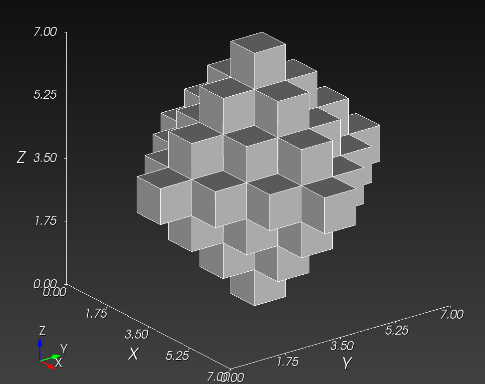 | 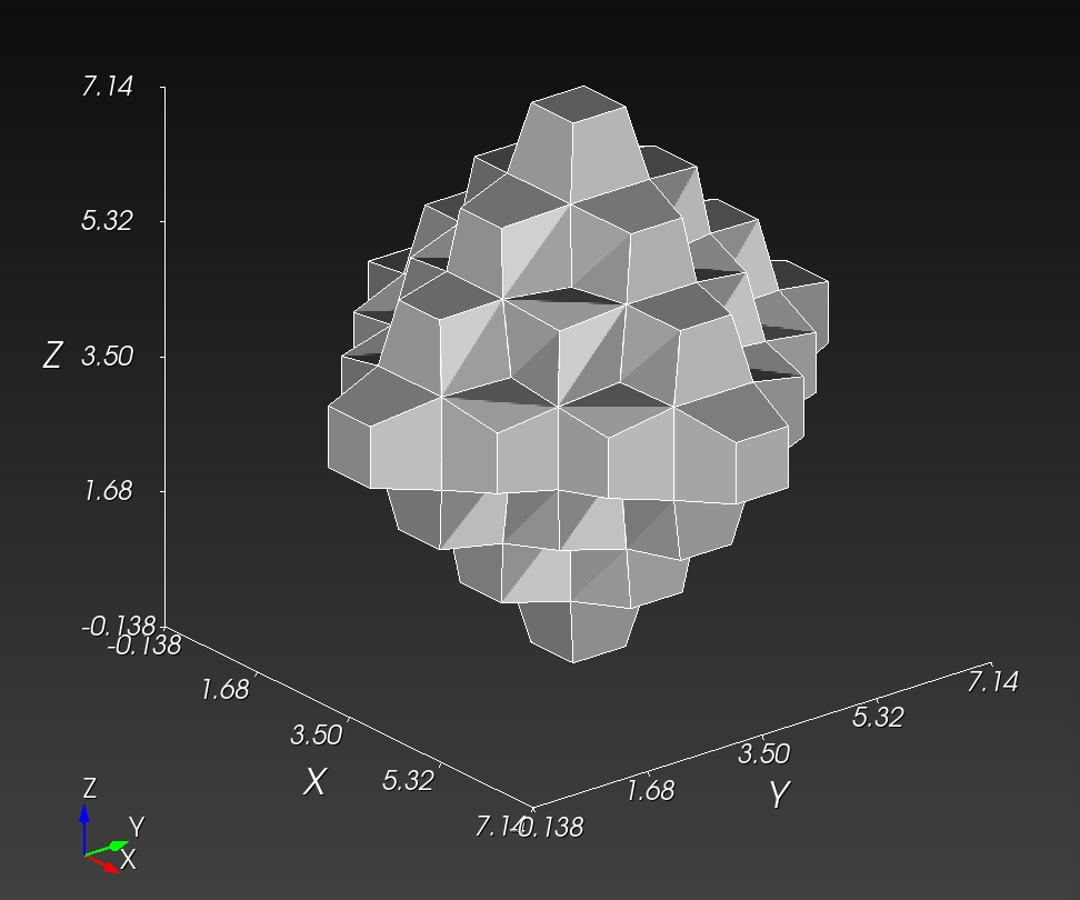 |
See the Smoothing Theory section for more information.
Isosurface
An isosurface can be generated from a segmentation using the tri command.
To create a mesh of the outer isosurfaces contained in the octahedron example:
automesh mesh tri -r 0 1 2 -i minimum_working_example/octahedron.npy -o minimum_working_example/octahedron.stl
    automesh 0.5.1
     Reading minimum_working_example/octahedron.npy
       Total 325.443µs
The surfaces are visualized below:
octahedron.stl in MeshLab | octahedron.stl in Cubit with cut plane |
|---|---|
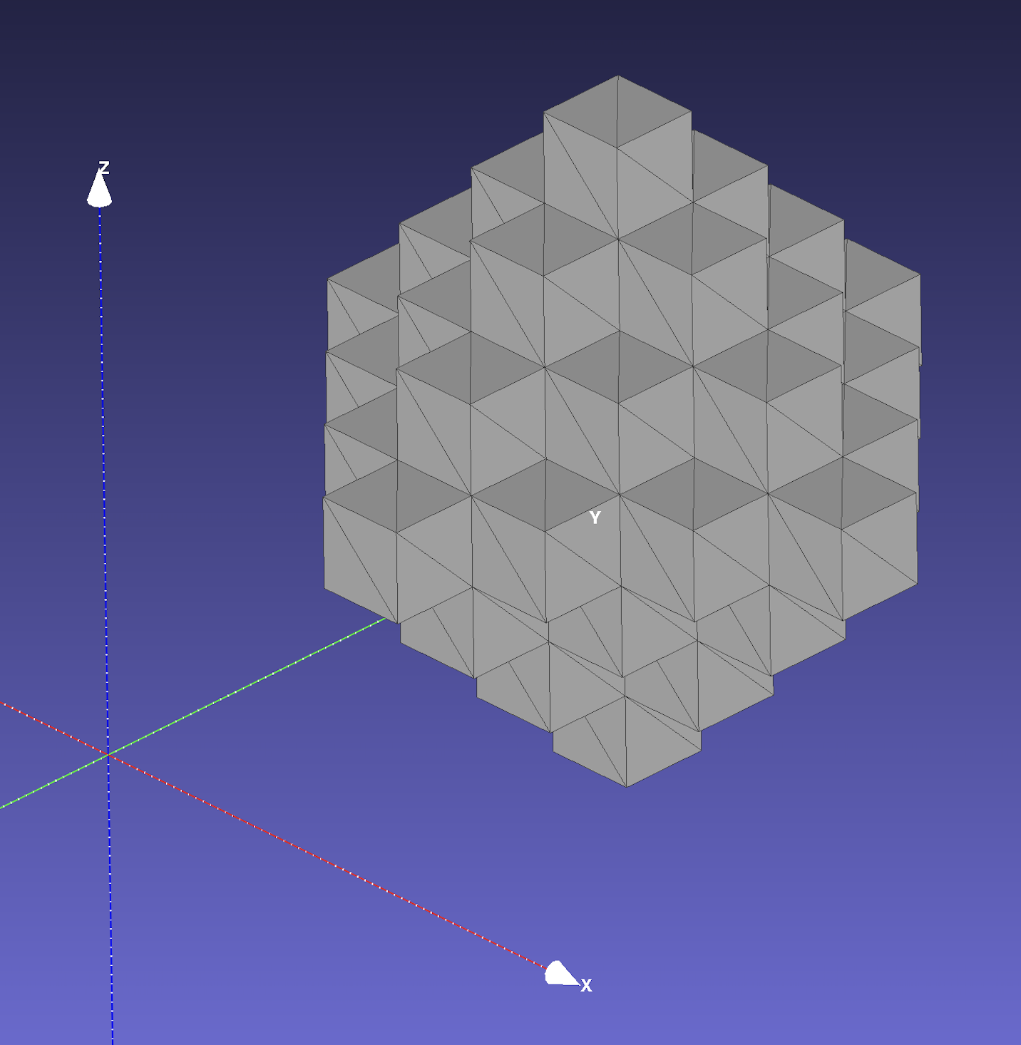 | 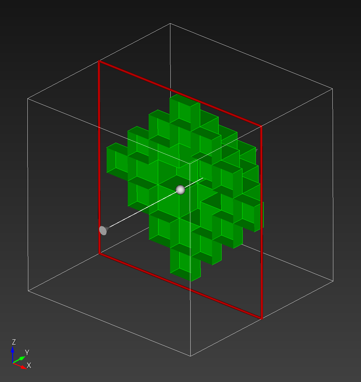 |
automesh creates an isosurface from the boundary faces of voxels. The
quadrilateral faces are divided into two triangles. The Isosurface section contains more details about alternative methods used to create an isosurface.
The Sphere with Shells section contains more examples of the command line interface.
Remark: Every
automeshcommand above also accepts--quietand--log FILE, to silence or record terminal output; see Global Options.
Command Line Interface
automesh is used primarily as a command line interface (CLI): a single
automesh binary with one subcommand per operation — convert,
defeature, diff, extract,
mesh, metrics, remesh,
segment, and smooth. Each subcommand
reads one or more input files and writes an output file.
automesh --help

     @@@@@@@@@@@@@@@@
      @@@@  @@@@@@@@@@
     @@@@  @@@@@@@@@@@    automesh: Automatic mesh generation
    @@@@  @@@@@@@@@@@@
      @@    @@    @@      v0.5.1 linux x86_64
      @@    @@    @@      build 667b104 2026-10-22T21:00:24+0000
    @@@@@@@@@@@@  @@@     Chad B. Hovey <chovey@sandia.gov>
    @@@@@@@@@@@  @@@@     Michael R. Buche <mrbuche@sandia.gov>
    @@@@@@@@@@ @@@@@ @
     @@@@@@@@@@@@@@@@

Usage: automesh [OPTIONS] [COMMAND]

Commands:
  convert    Converts between mesh or segmentation file types
  defeature  Defeatures and creates a new segmentation
  diff       Show the difference between two segmentations
  extract    Extracts a specified range of voxels from a segmentation
  mesh       Creates a finite element mesh from a segmentation
  metrics    Quality metrics for an existing finite element mesh
  partition  Partitions a mesh into parts, written as one exo file per part
  remesh     Applies isotropic remeshing to an existing mesh [default mode: uniform]
  segment    Creates a segmentation or voxelized mesh from an existing mesh
  smooth     Applies smoothing to an existing mesh
  help       Print this message or the help of the given subcommand(s)

Options:
  -h, --help     Print help
  -V, --version  Print version

Global options:
      --log <FILE>  Mirror terminal output to a log file
  -q, --quiet       Pass to quiet the terminal output
Global Options
Two options apply to every subcommand: --quiet and --log.
-
--quiet(-q) suppresses the terminal output — the banner, and each command'sReading/Meshing/Writing/Done/Totalprogress lines — while the command still runs normally. -
--log <FILE>mirrors that same terminal output into a file, with the color escape codes stripped so the file is plain text.automeshinserts a local date-time stamp before the file extension, so rerunning a command with the same--logpath never overwrites an earlier log:automesh --log run.log mesh hex -i octahedron.npy -o octahedron.inp -r 0Logging to run_2026-07-17T09-30-58-0600.logThe stamp is
YYYY-MM-DD(year-month-day),Tmarking the start of the time-of-day, thenHH-MM-SS(hour-minute-second, local time), followed by the local UTC offset-0600(six hours behind UTC — Mountain Daylight Time, in this example). Hyphens separate the hour, minute, and second instead of the more common:because:is not a legal filename character on Windows.
--quiet and --log are independent, so --quiet --log run.log runs silently
on the terminal while still writing the full log file — useful for scripted or
batch invocations where only a record of the run is wanted.
Convert
convert translates between file formats without changing the underlying
data: convert mesh translates between mesh formats (.exo, .inp, .mesh,
.off, .stl, .vtu), and convert segmentation translates between
segmentation formats (.npy, .spn, .vti).
automesh convert --help
Converts between mesh or segmentation file types

Usage: automesh convert [OPTIONS] <COMMAND>

Commands:
  mesh          Converts mesh file types (exo | inp | off | stl | vtu) -> (exo | inp | mesh | off | stl | vtu)
  segmentation  Converts segmentation file types (npy | spn) -> (npy | spn | vti)
  help          Print this message or the help of the given subcommand(s)

Options:
  -h, --help  Print help

Global options:
      --log <FILE>  Mirror terminal output to a log file
  -q, --quiet       Pass to quiet the terminal output
Convert Mesh
convert mesh automatically detects the element type(s) present in the
input file — hexahedral, tetrahedral, triangular, quadrilateral, wedge,
pyramidal, or a mix of these within the same mesh — and writes them to the
output format unchanged; there is no separate hex/tet/tri subcommand to
choose.
.stl and .off are the exceptions: both are surface-only formats.
.stl holds only 3D triangles. .off holds 3D triangles and
quadrilaterals.
- An
.stlor.offinput can be converted to any of the other mesh formats (.exo,.inp,.mesh,.vtu); the resulting mesh is composed of whatever surface elements the input held (triangles only, for.stl; triangles and/or quadrilaterals, for.off). - Any of the other mesh formats can be converted to
.stl, provided the input mesh is itself composed exclusively of triangular elements, or to.off, provided the input mesh is composed exclusively of triangular and/or quadrilateral elements. - A volumetric mesh (containing hexahedral, tetrahedral, wedge, or
pyramidal elements) cannot be converted to
.stlor.off.
automesh convert mesh --help
Converts mesh file types (exo | inp | off | stl | vtu) -> (exo | inp | mesh | off | stl | vtu)

Usage: automesh convert mesh [OPTIONS] --input <FILE> --output <FILE>

Options:
  -i, --input <FILE>   Mesh input file (exo | inp | off | stl | vtu)
  -o, --output <FILE>  Mesh output file (exo | inp | mesh | off | stl | vtu)
  -h, --help           Print help

Global options:
      --log <FILE>  Mirror terminal output to a log file
  -q, --quiet       Pass to quiet the terminal output
Convert Segmentation
automesh convert segmentation --help
Converts segmentation file types (npy | spn) -> (npy | spn | vti)

Usage: automesh convert segmentation [OPTIONS] --input <FILE> --output <FILE>

Options:
  -i, --input <FILE>   Segmentation input file (npy | spn)
  -o, --output <FILE>  Segmentation output file (npy | spn | vti)
  -x, --nelx <NEL>     Number of voxels in the x-direction (spn)
  -y, --nely <NEL>     Number of voxels in the y-direction (spn)
  -z, --nelz <NEL>     Number of voxels in the z-direction (spn)
  -h, --help           Print help

Global options:
      --log <FILE>  Mirror terminal output to a log file
  -q, --quiet       Pass to quiet the terminal output
Defeature
defeature removes small, undesired clusters of voxels using a voxel-count
threshold. A cluster of voxels, defined as two or more voxels that share a
face (edge and node sharing do not constitute a cluster) with count at or
above the threshold, is preserved, whereas a cluster with a count below the
threshold is eliminated through resorption into the surrounding material.
automesh defeature --help
Defeatures and creates a new segmentation

Usage: automesh defeature [OPTIONS] --input <FILE> --output <FILE> --min <MIN>

Options:
  -i, --input <FILE>   Segmentation input file (npy | spn)
  -o, --output <FILE>  Defeatured segmentation output file (npy | spn | vti)
  -m, --min <MIN>      Defeature clusters with less than MIN voxels
  -x, --nelx <NEL>     Number of voxels in the x-direction (spn)
  -y, --nely <NEL>     Number of voxels in the y-direction (spn)
  -z, --nelz <NEL>     Number of voxels in the z-direction (spn)
  -h, --help           Print help

Global options:
      --log <FILE>  Mirror terminal output to a log file
  -q, --quiet       Pass to quiet the terminal output
Examples
- Blobs — four synthetic circular blobs with random noise, illustrating how the threshold determines which clusters are preserved and which are resorbed.
Diff
diff compares two segmentations voxel-by-voxel and writes a new
segmentation encoding where the two inputs differ — useful for spotting
changes between two versions of the same domain, for example before and
after defeaturing or manual editing.
automesh diff --help
Show the difference between two segmentations

Usage: automesh diff [OPTIONS] --output <FILE>

Options:
  -i, --input <FILE> <FILE>  Segmentation input files (npy | spn)
  -o, --output <FILE>        Segmentation difference output file (npy | spn | vti)
  -x, --nelx <NEL>           Number of voxels in the x-direction (spn)
  -y, --nely <NEL>           Number of voxels in the y-direction (spn)
  -z, --nelz <NEL>           Number of voxels in the z-direction (spn)
  -h, --help                 Print help

Global options:
      --log <FILE>  Mirror terminal output to a log file
  -q, --quiet       Pass to quiet the terminal output
Extract
extract pulls a rectangular sub-range of voxels out of a larger
segmentation, given inclusive --xmin/--xmax, --ymin/--ymax, and
--zmin/--zmax bounds — useful for isolating a region of interest without
regenerating the whole domain.
automesh extract --help
Extracts a specified range of voxels from a segmentation

Usage: automesh extract [OPTIONS] --input <FILE> --output <FILE> --xmin <MIN> --xmax <MAX> --ymin <MIN> --ymax <MAX> --zmin <MIN> --zmax <MAX>

Options:
  -i, --input <FILE>   Segmentation input file (npy | spn)
  -o, --output <FILE>  Extracted segmentation output file (npy | spn | vti)
  -x, --nelx <NEL>     Number of voxels in the x-direction (spn)
  -y, --nely <NEL>     Number of voxels in the y-direction (spn)
  -z, --nelz <NEL>     Number of voxels in the z-direction (spn)
      --xmin <MIN>     Minimum voxel in the x-direction
      --xmax <MAX>     Maximum voxel in the x-direction
      --ymin <MIN>     Minimum voxel in the y-direction
      --ymax <MAX>     Maximum voxel in the y-direction
      --zmin <MIN>     Minimum voxel in the z-direction
      --zmax <MAX>     Maximum voxel in the z-direction
  -h, --help           Print help

Global options:
      --log <FILE>  Mirror terminal output to a log file
  -q, --quiet       Pass to quiet the terminal output
Mesh
mesh creates a finite element mesh from a segmentation. Its subcommands
create all-hexahedral (hex), hex-dominant (hexdom), polyhedral (poly),
all-tetrahedral (tet), and all-triangular (tri) meshes.
mesh hex produces an all-hexahedral (voxel) mesh. Its input is either a
segmentation, meshed directly into hexahedra, or a tessellation, converted
into hexahedra by octree dualization. For a tessellation, --uniform <SPACING> replaces the octree with a uniform lattice of cubes of the given
edge length, trimmed to the surface and buffered onto it exactly as the dual
is; the background is then ungraded, so --scale, --tolerance, --strong
and --levels no longer apply. An optional smooth subcommand can
be chained directly onto mesh hex. A further remesh subcommand can also
be chained after smooth — automesh mesh hex smooth remesh --help
succeeds, so the command line accepts it — but running it always fails.
remesh requires triangular connectivity, and a hex mesh has none, so the
run-time error is always connectivity contains a non-triangular block.
mesh tet produces an all-tetrahedral mesh from a tessellation. Every
element is a linear, four-noded tetrahedron. Ten-noded quadratic
tetrahedra are not supported. The input
must be an stl file. A segmentation input is rejected. The command builds
a tetrahedral background, six tetrahedra per cell of an octree fitted to the
surface. --uniform <SPACING> replaces the octree with a uniform lattice.
The command then trims the background to the surface and buffers it onto the
surface with a prism layer and a fit. An optional smooth subcommand can be
chained directly onto mesh tet. A further remesh subcommand parses but
always fails, with connectivity contains a non-triangular block, for the
same reason as mesh hex smooth remesh.
mesh tri produces an all-triangular isosurface mesh of the material
boundaries from a segmentation. An optional smooth subcommand can be
chained directly onto it, and a further remesh subcommand can be chained
after that — mesh tri smooth remesh works fully, since a triangular mesh
satisfies remesh's connectivity requirement.
automesh mesh --help
Creates a finite element mesh from a segmentation

Usage: automesh mesh [OPTIONS] <COMMAND>

Commands:
  hex     Creates an all-hexahedral mesh from a segmentation or tessellation
  hexdom  Creates a hex-dominant mesh from a tessellation, polyhedral at the boundary
  poly    Creates a polyhedral mesh from a tessellation
  tet     Creates an all-tetrahedral mesh from a tessellation
  tri     Creates all-triangular isosurface(s) from a segmentation
  help    Print this message or the help of the given subcommand(s)

Options:
  -h, --help  Print help

Global options:
      --log <FILE>  Mirror terminal output to a log file
  -q, --quiet       Pass to quiet the terminal output
Mesh Hex
automesh mesh hex --help
Creates an all-hexahedral mesh from a segmentation or tessellation

Usage: automesh mesh hex [OPTIONS] --input <FILE> --output <FILE> [COMMAND]

Commands:
  smooth  Applies smoothing to the mesh before output
  help    Print this message or the help of the given subcommand(s)

Options:
  -i, --input <FILE>
          Segmentation (npy | spn) or tessellation (stl) input file

  -o, --output <FILE>
          Mesh output file (exo | inp | mesh | off | stl | vtu)

  -d, --defeature <NUM>
          Defeature clusters with less than NUM voxels

  -x, --nelx <NEL>
          Number of voxels in the x-direction (spn)

  -y, --nely <NEL>
          Number of voxels in the y-direction (spn)

  -z, --nelz <NEL>
          Number of voxels in the z-direction (spn)

  -r, --remove <ID>...
          Voxel IDs to remove from the mesh (npy | spn)

      --xscale <SCALE>
          Scaling (> 0.0) in the x-direction, applied before translation

          [default: 1]

      --yscale <SCALE>
          Scaling (> 0.0) in the y-direction, applied before translation

          [default: 1]

      --zscale <SCALE>
          Scaling (> 0.0) in the z-direction, applied before translation

          [default: 1]

      --xtranslate <VAL>
          Translation in the x-direction

          [default: 0]

      --ytranslate <VAL>
          Translation in the y-direction

          [default: 0]

      --ztranslate <VAL>
          Translation in the z-direction

          [default: 0]

  -s, --scale <SCALE>
          Octree refinement scale for dualizing a tessellation (stl) input

          [default: 5]

  -u, --uniform <SPACING>
          Uniform mesh of the given element size instead of an octree (stl)

  -t, --tolerance <TOL>
          Chord-error tolerance for curvature-driven refinement [default: disabled]

      --strong
          Uses strong balancing instead of the default weak balancing

      --inflate
          Cuts the uniform lattice with marching cubes and inflates it onto the surface (stl)

      --marching
          Cuts the uniform lattice with marching cubes, leaving the boundary as cut (stl)

      --snap
          Snaps the buffer layer onto the surface instead of a soft fit

      --pyramids <MSJ>
          Replaces shell hexahedra below this minimum scaled Jacobian along features with pyramids and refits, snapping both fits under --snap [default: disabled]

  -l, --levels <NUM>
          Level difference allowed between neighboring octree cells (poly)

          [default: 1]

      --metrics <FILE>
          Quality metrics output file (csv | npy)

      --cubes <METHOD>
          Isosurface method for triangles from a segmentation (tri)

          Possible values:
          - cuberille: Faces of the voxels, shared between materials
          - marching:  Smooth isosurface of each material

          [default: cuberille]

  -h, --help
          Print help (see a summary with '-h')

Global options:
      --log <FILE>
          Mirror terminal output to a log file

  -q, --quiet
          Pass to quiet the terminal output
Mesh Tet
automesh mesh tet --help
Creates an all-tetrahedral mesh from a tessellation

Usage: automesh mesh tet [OPTIONS] --input <FILE> --output <FILE> [COMMAND]

Commands:
  smooth  Applies smoothing to the mesh before output
  help    Print this message or the help of the given subcommand(s)

Options:
  -i, --input <FILE>
          Segmentation (npy | spn) or tessellation (stl) input file

  -o, --output <FILE>
          Mesh output file (exo | inp | mesh | off | stl | vtu)

  -d, --defeature <NUM>
          Defeature clusters with less than NUM voxels

  -x, --nelx <NEL>
          Number of voxels in the x-direction (spn)

  -y, --nely <NEL>
          Number of voxels in the y-direction (spn)

  -z, --nelz <NEL>
          Number of voxels in the z-direction (spn)

  -r, --remove <ID>...
          Voxel IDs to remove from the mesh (npy | spn)

      --xscale <SCALE>
          Scaling (> 0.0) in the x-direction, applied before translation

          [default: 1]

      --yscale <SCALE>
          Scaling (> 0.0) in the y-direction, applied before translation

          [default: 1]

      --zscale <SCALE>
          Scaling (> 0.0) in the z-direction, applied before translation

          [default: 1]

      --xtranslate <VAL>
          Translation in the x-direction

          [default: 0]

      --ytranslate <VAL>
          Translation in the y-direction

          [default: 0]

      --ztranslate <VAL>
          Translation in the z-direction

          [default: 0]

  -s, --scale <SCALE>
          Octree refinement scale for dualizing a tessellation (stl) input

          [default: 5]

  -u, --uniform <SPACING>
          Uniform mesh of the given element size instead of an octree (stl)

  -t, --tolerance <TOL>
          Chord-error tolerance for curvature-driven refinement [default: disabled]

      --strong
          Uses strong balancing instead of the default weak balancing

      --inflate
          Cuts the uniform lattice with marching cubes and inflates it onto the surface (stl)

      --marching
          Cuts the uniform lattice with marching cubes, leaving the boundary as cut (stl)

      --snap
          Snaps the buffer layer onto the surface instead of a soft fit

      --pyramids <MSJ>
          Replaces shell hexahedra below this minimum scaled Jacobian along features with pyramids and refits, snapping both fits under --snap [default: disabled]

  -l, --levels <NUM>
          Level difference allowed between neighboring octree cells (poly)

          [default: 1]

      --metrics <FILE>
          Quality metrics output file (csv | npy)

      --cubes <METHOD>
          Isosurface method for triangles from a segmentation (tri)

          Possible values:
          - cuberille: Faces of the voxels, shared between materials
          - marching:  Smooth isosurface of each material

          [default: cuberille]

  -h, --help
          Print help (see a summary with '-h')

Global options:
      --log <FILE>
          Mirror terminal output to a log file

  -q, --quiet
          Pass to quiet the terminal output
mesh tet shares its options with mesh hex, so --help lists options that
apply to other subcommands. Passing --marching without --uniform fails at
the command line. Passing --levels fails with
Dualization requires 2:1 balancing, so levels applies to mesh poly only.
Mesh Tri
automesh mesh tri --help
Creates all-triangular isosurface(s) from a segmentation

Usage: automesh mesh tri [OPTIONS] --input <FILE> --output <FILE> [COMMAND]

Commands:
  smooth  Applies smoothing to the mesh before output
  help    Print this message or the help of the given subcommand(s)

Options:
  -i, --input <FILE>
          Segmentation (npy | spn) or tessellation (stl) input file

  -o, --output <FILE>
          Mesh output file (exo | inp | mesh | off | stl | vtu)

  -d, --defeature <NUM>
          Defeature clusters with less than NUM voxels

  -x, --nelx <NEL>
          Number of voxels in the x-direction (spn)

  -y, --nely <NEL>
          Number of voxels in the y-direction (spn)

  -z, --nelz <NEL>
          Number of voxels in the z-direction (spn)

  -r, --remove <ID>...
          Voxel IDs to remove from the mesh (npy | spn)

      --xscale <SCALE>
          Scaling (> 0.0) in the x-direction, applied before translation

          [default: 1]

      --yscale <SCALE>
          Scaling (> 0.0) in the y-direction, applied before translation

          [default: 1]

      --zscale <SCALE>
          Scaling (> 0.0) in the z-direction, applied before translation

          [default: 1]

      --xtranslate <VAL>
          Translation in the x-direction

          [default: 0]

      --ytranslate <VAL>
          Translation in the y-direction

          [default: 0]

      --ztranslate <VAL>
          Translation in the z-direction

          [default: 0]

  -s, --scale <SCALE>
          Octree refinement scale for dualizing a tessellation (stl) input

          [default: 5]

  -u, --uniform <SPACING>
          Uniform mesh of the given element size instead of an octree (stl)

  -t, --tolerance <TOL>
          Chord-error tolerance for curvature-driven refinement [default: disabled]

      --strong
          Uses strong balancing instead of the default weak balancing

      --inflate
          Cuts the uniform lattice with marching cubes and inflates it onto the surface (stl)

      --marching
          Cuts the uniform lattice with marching cubes, leaving the boundary as cut (stl)

      --snap
          Snaps the buffer layer onto the surface instead of a soft fit

      --pyramids <MSJ>
          Replaces shell hexahedra below this minimum scaled Jacobian along features with pyramids and refits, snapping both fits under --snap [default: disabled]

  -l, --levels <NUM>
          Level difference allowed between neighboring octree cells (poly)

          [default: 1]

      --metrics <FILE>
          Quality metrics output file (csv | npy)

      --cubes <METHOD>
          Isosurface method for triangles from a segmentation (tri)

          Possible values:
          - cuberille: Faces of the voxels, shared between materials
          - marching:  Smooth isosurface of each material

          [default: cuberille]

  -h, --help
          Print help (see a summary with '-h')

Global options:
      --log <FILE>
          Mirror terminal output to a log file

  -q, --quiet
          Pass to quiet the terminal output
Mesh Hex Smooth
automesh mesh hex smooth --help
Applies smoothing to the mesh before output

Usage: automesh mesh hex --input <FILE> --output <FILE> smooth [OPTIONS] [COMMAND]

Commands:
  remesh  Applies remeshing to the mesh before output [default mode: uniform]
  help    Print this message or the help of the given subcommand(s)

Options:
  -n, --iterations <NUM>  Number of smoothing iterations [default: 20]
  -m, --method <NAME>     Smoothing method [default: Taubin] [possible values: Laplace, Taubin]
  -k, --pass-band <FREQ>  Pass-band frequency (for Taubin only) [default: 0.1]
  -s, --scale <SCALE>     Scaling parameter for all smoothing methods [default: 0.6307]
  -b, --hierarchical      Enables hierarchical smoothing
  -h, --help              Print help

Global options:
      --log <FILE>  Mirror terminal output to a log file
  -q, --quiet       Pass to quiet the terminal output
mesh hex smooth accepts a further remesh subcommand at the command line
(automesh mesh hex smooth remesh --help succeeds), but running it always
fails — remesh requires triangular connectivity, and a hex mesh has none.
Remeshing after smoothing is only meaningful for mesh tri, below.
Mesh Tet Smooth
automesh mesh tet smooth --help
Applies smoothing to the mesh before output

Usage: automesh mesh tet --input <FILE> --output <FILE> smooth [OPTIONS] [COMMAND]

Commands:
  remesh  Applies remeshing to the mesh before output [default mode: uniform]
  help    Print this message or the help of the given subcommand(s)

Options:
  -n, --iterations <NUM>  Number of smoothing iterations [default: 20]
  -m, --method <NAME>     Smoothing method [default: Taubin] [possible values: Laplace, Taubin]
  -k, --pass-band <FREQ>  Pass-band frequency (for Taubin only) [default: 0.1]
  -s, --scale <SCALE>     Scaling parameter for all smoothing methods [default: 0.6307]
  -b, --hierarchical      Enables hierarchical smoothing
  -h, --help              Print help

Global options:
      --log <FILE>  Mirror terminal output to a log file
  -q, --quiet       Pass to quiet the terminal output
mesh tet smooth accepts a further remesh subcommand at the command line,
but running it always fails. remesh requires triangular connectivity.
Mesh Tri Smooth
automesh mesh tri smooth --help
Applies smoothing to the mesh before output

Usage: automesh mesh tri --input <FILE> --output <FILE> smooth [OPTIONS] [COMMAND]

Commands:
  remesh  Applies remeshing to the mesh before output [default mode: uniform]
  help    Print this message or the help of the given subcommand(s)

Options:
  -n, --iterations <NUM>  Number of smoothing iterations [default: 20]
  -m, --method <NAME>     Smoothing method [default: Taubin] [possible values: Laplace, Taubin]
  -k, --pass-band <FREQ>  Pass-band frequency (for Taubin only) [default: 0.1]
  -s, --scale <SCALE>     Scaling parameter for all smoothing methods [default: 0.6307]
  -b, --hierarchical      Enables hierarchical smoothing
  -h, --help              Print help

Global options:
      --log <FILE>  Mirror terminal output to a log file
  -q, --quiet       Pass to quiet the terminal output
Mesh Tri Smooth Remesh
automesh mesh tri smooth remesh --help
Applies remeshing to the mesh before output [default mode: uniform]

Usage: automesh mesh tri smooth remesh [OPTIONS] [COMMAND]

Commands:
  uniform   Uniform target edge length over the whole mesh
  adaptive  Curvature-adaptive target edge length
  help      Print this message or the help of the given subcommand(s)

Options:
  -h, --help  Print help

Global options:
      --log <FILE>  Mirror terminal output to a log file
  -q, --quiet       Pass to quiet the terminal output
Examples
- Torus — a genus-1 solid meshed and smoothed in
a single chained
mesh hex smoothcommand, comparing raw vs. smoothed element quality, and reproducing themesh hex smooth remeshfailure documented above. - Remeshed unit sphere —
mesh hexdualizing a triangular surface into a solid all-hexahedral volume, and how the--scaleoctree depth affects element quality. - Unit sphere and the
Stanford bunny —
mesh tri smooth remeshworked in full, as part of the Remesh examples.
Metrics
metrics evaluates element quality for an existing finite element mesh and
writes one quality value per element (as csv or npy), so mesh quality can
be assessed before analysis. Poorly shaped elements — thin, skewed, or
inverted — degrade the accuracy and stability of a simulation, and these
metrics quantify that shape quality.
automesh metrics --help
Quality metrics for an existing finite element mesh

Usage: automesh metrics [OPTIONS] --input <FILE> --output <FILE>

Options:
  -i, --input <FILE>   Mesh input file (exo | inp | off | stl | vtu)
  -o, --output <FILE>  Quality metrics output file (csv | npy)
  -h, --help           Print help

Global options:
      --log <FILE>  Mirror terminal output to a log file
  -q, --quiet       Pass to quiet the terminal output
The available metrics depend on the element type. Each is defined, with acceptable ranges from Knupp et al.1, in Theory:
- Hexahedral metrics — for eight-node brick elements: maximum edge ratio, minimum scaled Jacobian, maximum skew, and element volume.
- Tetrahedral metrics — for four-node tetrahedral elements: maximum edge ratio, minimum scaled Jacobian, maximum skew, and element volume.
- Triangular metrics — for three-node triangular surface elements: maximum edge ratio, minimum scaled Jacobian, maximum skew, element area, and minimum angle.
-
Knupp PM, Ernst CD, Thompson DC, Stimpson CJ, Pebay PP. The verdict geometric quality library. SAND2007-1751. Sandia National Laboratories (SNL), Albuquerque, NM, and Livermore, CA (United States); 2006 Mar 1. link ↩
Remesh
remesh applies isotropic surface remeshing to an existing triangular
surface mesh. Starting from the input triangulation, it iteratively splits,
collapses, flips, and smooths edges to drive every edge toward a target edge
length. The result is a surface mesh with more uniform, better-quality
triangles, either coarsened or refined relative to the input.
automesh remesh --help
Applies isotropic remeshing to an existing mesh [default mode: uniform]

Usage: automesh remesh [OPTIONS] --input <FILE> --output <FILE> [COMMAND]

Commands:
  uniform   Uniform target edge length over the whole mesh
  adaptive  Curvature-adaptive target edge length
  help      Print this message or the help of the given subcommand(s)

Options:
  -i, --input <FILE>   Mesh input file (exo | inp | off | stl | vtu)
  -o, --output <FILE>  Mesh output file (exo | inp | mesh | off | stl | vtu)
  -h, --help           Print help

Global options:
      --log <FILE>  Mirror terminal output to a log file
  -q, --quiet       Pass to quiet the terminal output
Remeshing reads and writes surface (triangular) mesh formats; see the --input
and --output formats listed in the help above. STL input may be either
ASCII or binary — the encoding is detected automatically. STL output is
always written binary.
remesh runs in one of two sizing modes, uniform and adaptive.
Remesh Uniform
A single target edge length is applied over the whole mesh; use it to coarsen or refine a surface to a chosen resolution.
automesh remesh uniform --help
Uniform target edge length over the whole mesh

Usage: automesh remesh --input <FILE> --output <FILE> uniform [OPTIONS]

Options:
  -n, --iterations <NUM>  Number of remeshing iterations [default: 5]
  -s, --size <SIZE>       Target edge length [default: mean edge length]
  -h, --help              Print help

Global options:
      --log <FILE>  Mirror terminal output to a log file
  -q, --quiet       Pass to quiet the terminal output
--iterations <NUM>— number of remeshing passes (default: 5). More passes bring the mesh closer to the target edge length.--size <SIZE>— the target edge length. When omitted, the mean edge length of the input mesh is used, which regularizes the mesh without significantly changing its resolution.
Remesh Adaptive
The target edge length varies with local surface curvature, between a --minimum
and --maximum, so curved regions are refined and flat regions are coarsened.
automesh remesh adaptive --help
Curvature-adaptive target edge length

Usage: automesh remesh --input <FILE> --output <FILE> adaptive [OPTIONS] --minimum <MIN> --maximum <MAX>

Options:
  -n, --iterations <NUM>  Number of remeshing iterations [default: 5]
      --minimum <MIN>     Minimum edge length
      --maximum <MAX>     Maximum edge length
  -t, --tolerance <TOL>   Curvature tolerance [default: 0.1]
  -g, --gradation <GRAD>  Size gradation factor [default: 0.5]
  -h, --help              Print help

Global options:
      --log <FILE>  Mirror terminal output to a log file
  -q, --quiet       Pass to quiet the terminal output
--iterations <NUM>— number of remeshing passes (default: 5).--minimum <MIN>— minimum edge length, used in high-curvature regions (required).--maximum <MAX>— maximum edge length, used in flat regions (required).--tolerance <TOL>— curvature tolerance controlling how strongly curvature drives the local edge length (default: 0.1).--gradation <GRAD>— size gradation factor controlling how smoothly the edge length transitions between the minimum and maximum (default: 0.5).
Examples
Two worked examples apply these options and illustrate the results:
- Unit sphere — an analytic unit sphere: mesh statistics, closed-surface relationships, uniform vs. adaptive sizing, and the effect of the number of iterations.
- Stanford bunny — a real scanned surface with
varying curvature, where uniform and adaptive sizing differ visibly, with a
walkthrough of every
remeshparameter.
Segment
segment is the inverse of mesh: it samples an existing mesh back into a
voxelized segmentation or mesh, at a chosen element size. The element type
(hex, tet, or tri) is detected automatically from the input mesh file;
there is no separate hex/tet/tri subcommand to choose.
automesh segment --help
Creates a segmentation or voxelized mesh from an existing mesh

Usage: automesh segment [OPTIONS] --input <FILE> --output <FILE> --size <NUM>

Options:
  -i, --input <FILE>    Mesh input file (exo | inp | off | stl | vtu)
  -o, --output <FILE>   Segmentation (npy | spn | vti) or mesh (exo | inp | mesh | vtu) output file
  -g, --grid <NUM>      Grid length for sampling within each element (currently unused) [default: 1]
  -s, --size <NUM>      Element size which is the side length
  -r, --remove <ID>...  Block IDs to remove from the segmentation
  -h, --help            Print help

Global options:
      --log <FILE>  Mirror terminal output to a log file
  -q, --quiet       Pass to quiet the terminal output
Sample Points
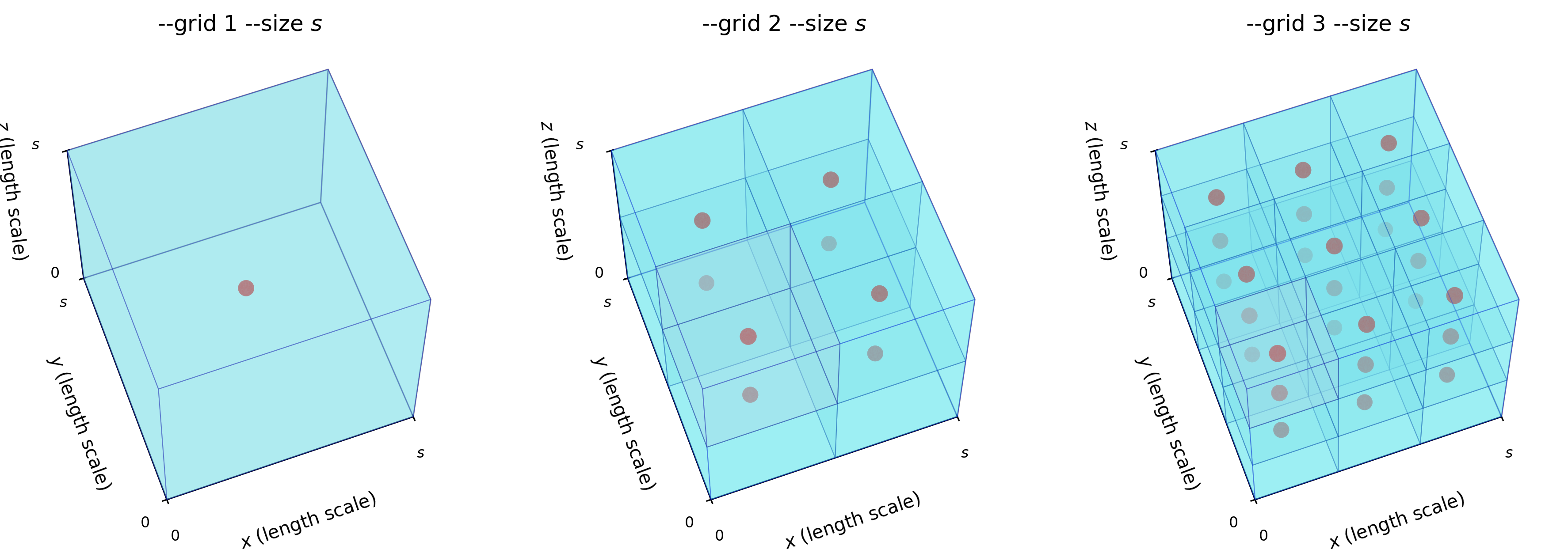
The input mesh is queried for its material composition for
--grid 1: at a single discrete sample point located at the center of a voxel,--grid 2: at eight discrete sample points located in a2x2x2arrangement within subdivided cells of the voxel,--grid 3: at 27 discrete sample points located within a3x3x3arrangement within subdivided cells of the voxel,- and so on.
The --grid and --size options are illustrated below for three successive grid sizes:
Smooth
smooth adjusts the positions of the nodes in a finite element mesh, using
either Laplacian or Taubin smoothing. Laplacian smoothing moves each node
toward the average
position of its neighbors, which reduces high-frequency noise but shrinks
the domain. Taubin smoothing is a two-pass extension of Laplacian
smoothing — a smoothing pass followed by a re-expansion pass — that avoids
that shrinkage. Hierarchical control can restrict which nodes are free to
move, so a mesh's exterior or interface geometry can be preserved during
smoothing. The element type is detected automatically from the input mesh
file; there is no separate hex/tri subcommand to choose. See
Smoothing Theory for the full derivations.
automesh smooth --help
Applies smoothing to an existing mesh

Usage: automesh smooth [OPTIONS] --input <FILE> --output <FILE> [COMMAND]

Commands:
  remesh  Applies remeshing to the mesh before output [default mode: uniform]
  help    Print this message or the help of the given subcommand(s)

Options:
  -i, --input <FILE>      Mesh input file (exo | inp | off | stl | vtu)
  -o, --output <FILE>     Smoothed mesh output file (exo | inp | mesh | off | stl | vtu)
  -n, --iterations <NUM>  Number of smoothing iterations [default: 20]
  -m, --method <NAME>     Smoothing method [default: Taubin] [possible values: Laplace, Taubin]
  -k, --pass-band <FREQ>  Pass-band frequency (for Taubin only) [default: 0.1]
  -s, --scale <SCALE>     Scaling parameter for all smoothing methods [default: 0.6307]
  -b, --hierarchical      Enables hierarchical smoothing
      --metrics <FILE>    Quality metrics output file (csv | npy)
  -h, --help              Print help

Global options:
      --log <FILE>  Mirror terminal output to a log file
  -q, --quiet       Pass to quiet the terminal output
Smooth Remesh
An optional remesh subcommand can be chained directly onto smoothing,
regardless of the input mesh's element type:
automesh smooth remesh --help
Applies remeshing to the mesh before output [default mode: uniform]

Usage: automesh smooth --input <FILE> --output <FILE> remesh [OPTIONS] [COMMAND]

Commands:
  uniform   Uniform target edge length over the whole mesh
  adaptive  Curvature-adaptive target edge length
  help      Print this message or the help of the given subcommand(s)

Options:
  -h, --help  Print help

Global options:
      --log <FILE>  Mirror terminal output to a log file
  -q, --quiet       Pass to quiet the terminal output
Examples
- Laplace — a two-element example worked by hand, showing neighborhoods and node positions across iterations of Laplace smoothing.
- Laplace with Hierarchical Control — the Bracket example, contrasting unrestricted Laplace smoothing with hierarchically-controlled smoothing that preserves prescribed geometry.
- Taubin — a noised hexahedral sphere mesh, compared directly against Taubin's original paper figure.
- Python Visualization — the source scripts used to generate the Laplace and hierarchical Laplace figures above.
Examples
Following are examples created with automesh. Unit Tests
and Spheres illustrate the segmentation and
meshing basics on small, hand-built cases. The remaining pages are worked
examples for specific commands: Blobs for
defeature; a torus for chained mesh hex smooth,
and a remeshed unit sphere for mesh hex
dualization of a tessellation; a unit sphere and
the Stanford bunny for remesh; and
Laplace,
Laplace with hierarchical control,
and Taubin smoothing, with the
Python source used to generate
the smoothing figures.
Unit Tests
The following illustrates a subset of the cases used to validate the code
implementation's voxel-to-mesh node numbering. Validation of these cases is
performed by a pytest suite rather than cargo test; for the complete set
of gold-value checks, see
examples_test.py.
The Python code used to generate the figures on this page is included
below, alongside examples_test.py in full.
Remark: We use the convention np when importing numpy as follows:
The NumPy import
import numpy as np
Single
The minimum working example (MWE) is a single voxel, used to create a single mesh consisting of one block consisting of a single element. The NumPy input single.npy contains the following segmentation:
The single.npy segmentation
segmentation = np.array(
    [
        [
            [ 11, ],
        ],
    ],
    dtype=np.uint8,
)
where the segmentation 11 denotes block 11 in the finite element mesh.
Remark: Serialization (write and read)
| Write | Read |
|---|---|
Use the np.save command to serialize the segmentation a .npy file | Use the np.load command to deserialize the segmentation from a .npy file |
Example: Write the data in segmentation to a file called seg.npynp.save("seg.npy", segmentation) | Example: Read the data from the file seg.npy to a variable called loaded_arrayloaded_array = np.load("seg.npy") |
Equivalently, the single.spn contains a single integer:
The .spn segmentation
11 # x:1 y:1 z:1
The resulting finite element mesh is visualized is shown in the following figure:
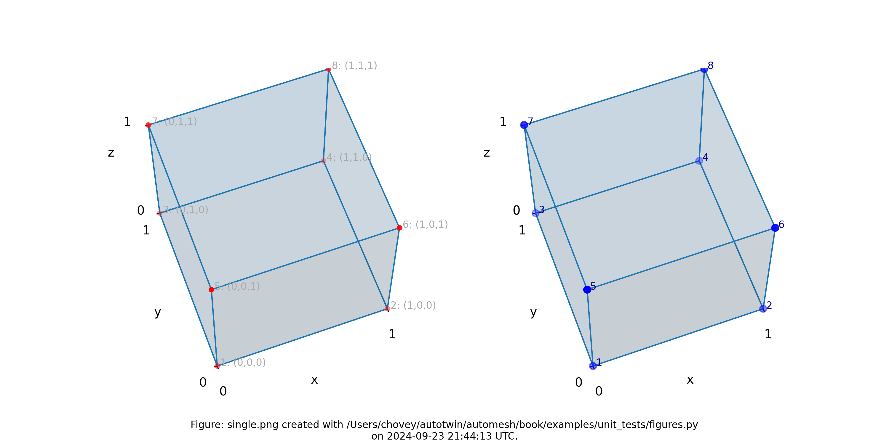
Figure 4.1-1: The single.png visualization, (left) lattice node numbers, (right)
mesh node numbers. Lattice node numbers appear in gray, with (x, y, z)
indices in parenthesis. The right-hand rule is used. Lattice coordinates
start at (0, 0, 0), and proceed along the x-axis, then
the y-axis, and then the z-axis.
The finite element mesh local node numbering map to the following global node numbers identically, and :
The local-to-global node map
[1, 2, 4, 3, 5, 6, 8, 7]
->
[1, 2, 4, 3, 5, 6, 8, 7]
which is a special case not typically observed, as shown in more complex examples below.
Remark: Input .npy and .spn files for the examples below can be found on the repository at automesh/tests/input.
Double
The next level of complexity example is a two-voxel domain, used to create
a single block composed of two finite elements. We test propagation in
both the x and y directions. The figures below show these two
meshes.
Double X
The .spn segmentation
11   #  x:1  y:1  z:1
11   #    2    1    1
where the segmentation 11 denotes block 11 in the finite element mesh.
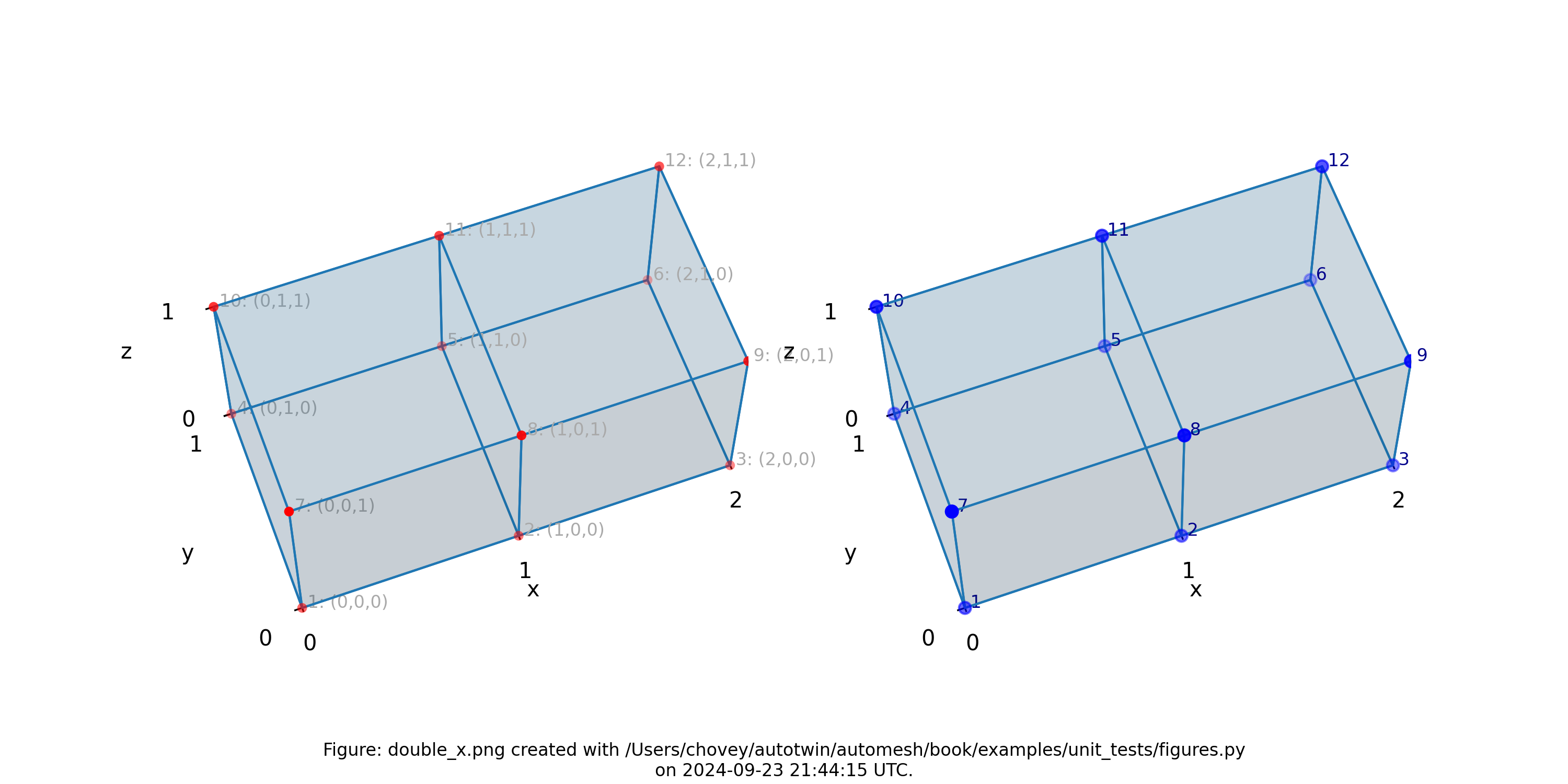
Figure 4.1-2: Mesh composed of a single block with two elements, propagating along
the x-axis, (left) lattice node numbers, (right) mesh node numbers.
Double Y
The .spn segmentation
11   #  x:1  y:1  z:1
11   #    1    2    1
where the segmentation 11 denotes block 11 in the finite element mesh.
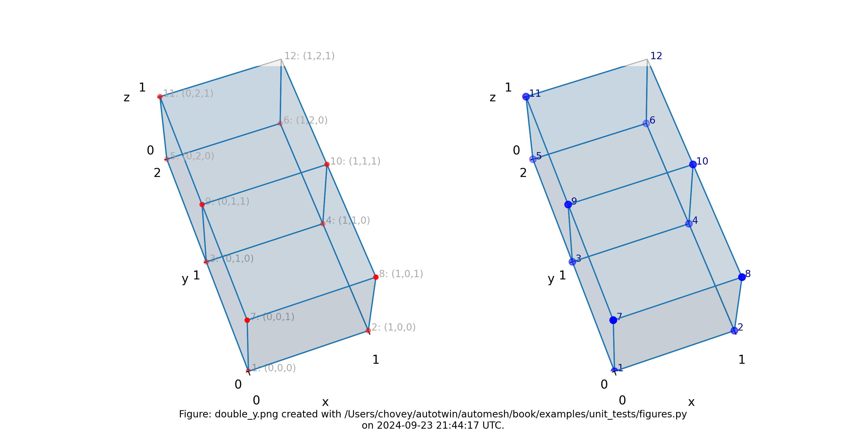
Figure 4.1-3: Mesh composed of a single block with two elements, propagating along
the y-axis, (left) lattice node numbers, (right) mesh node numbers.
Triple
The .spn segmentation
11   #  x:1  y:1  z:1
11   #    2    1    1
11   #    3    1    1
where the segmentation 11 denotes block 11 in the finite element mesh.
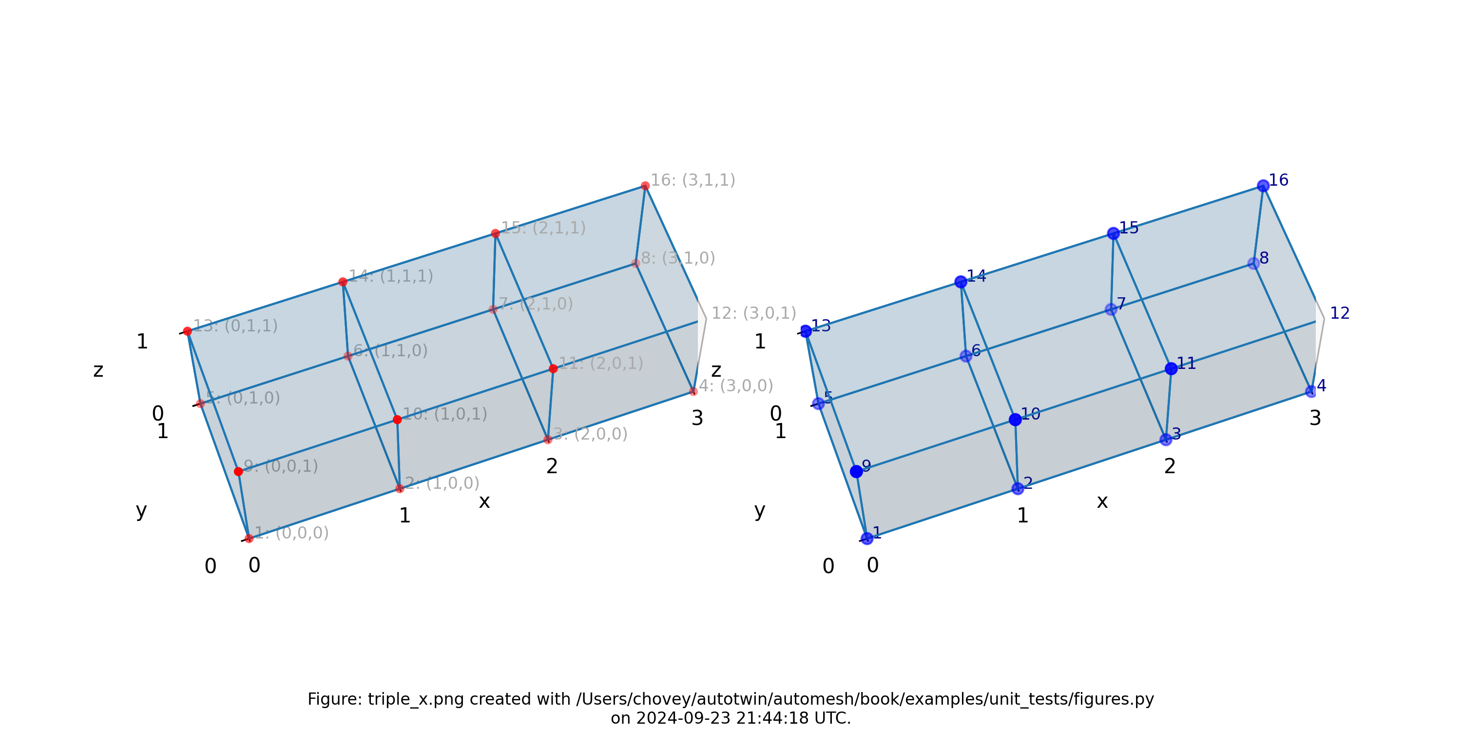
Figure 4.1-4: Mesh composed of a single block with three elements, propagating along
the x-axis, (left) lattice node numbers, (right) mesh node numbers.
Quadruple
The .spn segmentation
11   #  x:1  y:1  z:1
11   #    2    1    1
11   #    3    1    1
11   #    4    1    1
where the segmentation 11 denotes block 11 in the finite element mesh.
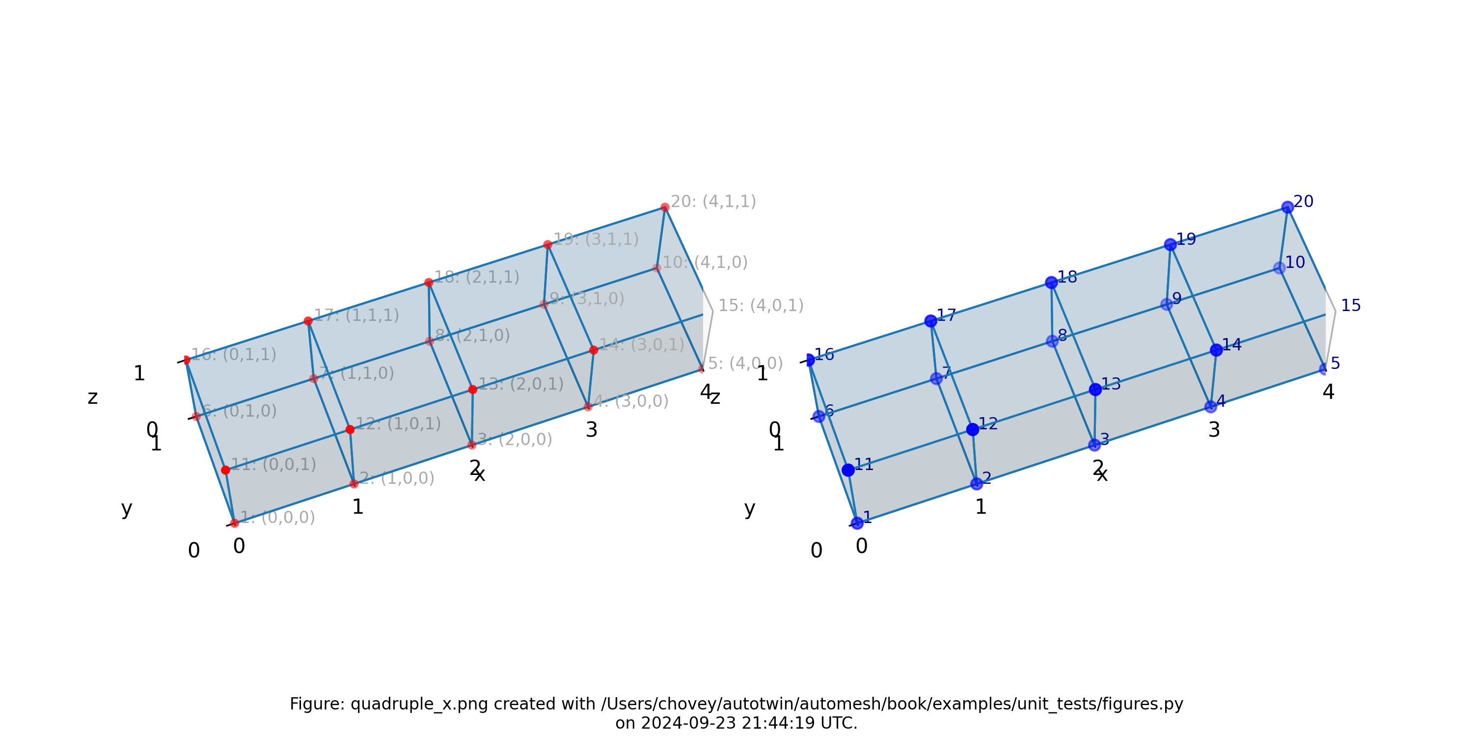
Figure 4.1-5: Mesh composed of a single block with four elements, propagating along
the x-axis, (left) lattice node numbers, (right) mesh node numbers.
Quadruple with Voids
The .spn segmentation
99   #  x:1  y:1  z:1
0    #    2    1    1
0    #    3    1    1
99   #    4    1    1
where the segmentation 99 denotes block 99 in the finite element mesh, and segmentation 0 is excluded from the mesh.
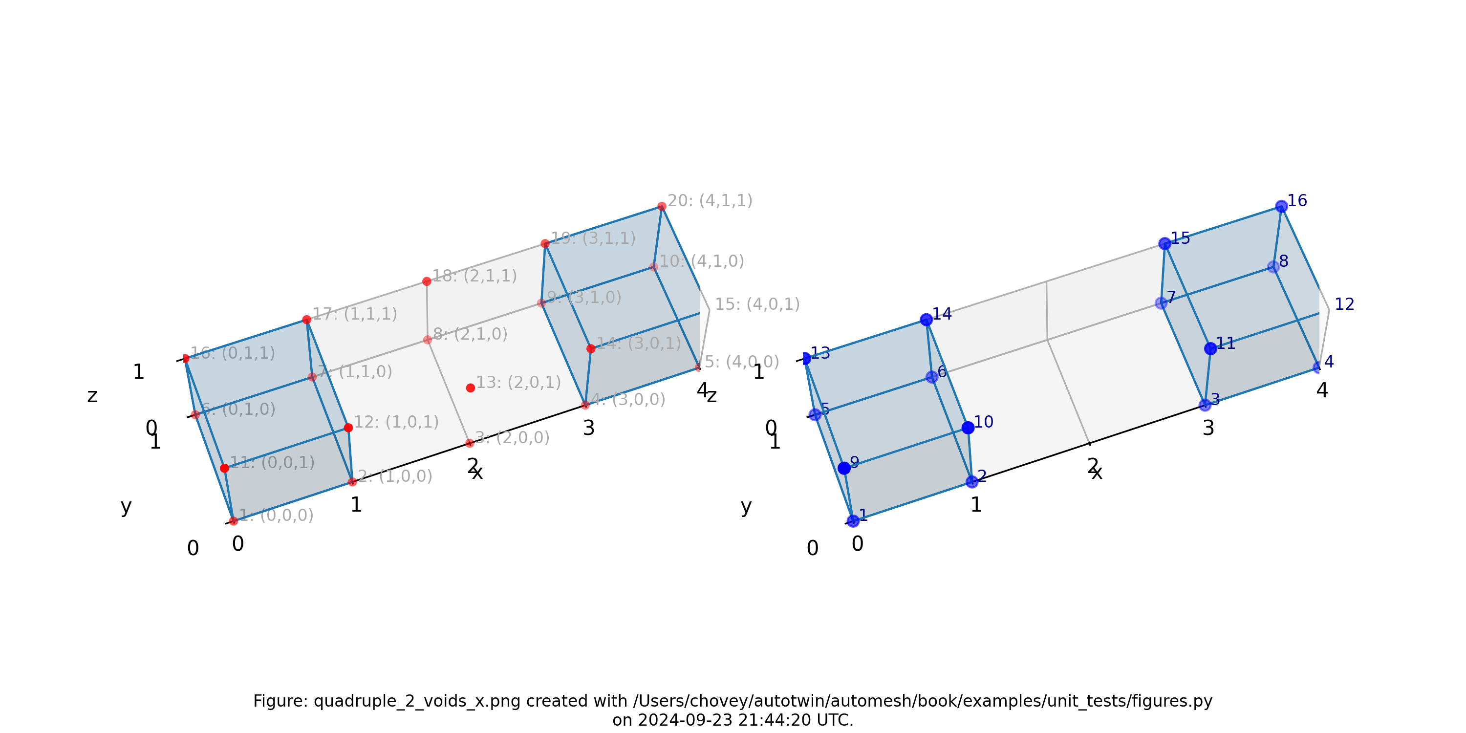
Figure 4.1-6: Mesh composed of a single block with two elements, propagating along
the x-axis and two voids, (left) lattice node numbers, (right) mesh node
numbers.
Quadruple with Two Blocks
The .spn segmentation
100  #  x:1  y:1  z:1
101  #    2    1    1
101  #    3    1    1
100  #    4    1    1
where the segmentation 100 and 101 denotes block 100 and 101,
respectively in the finite element mesh.
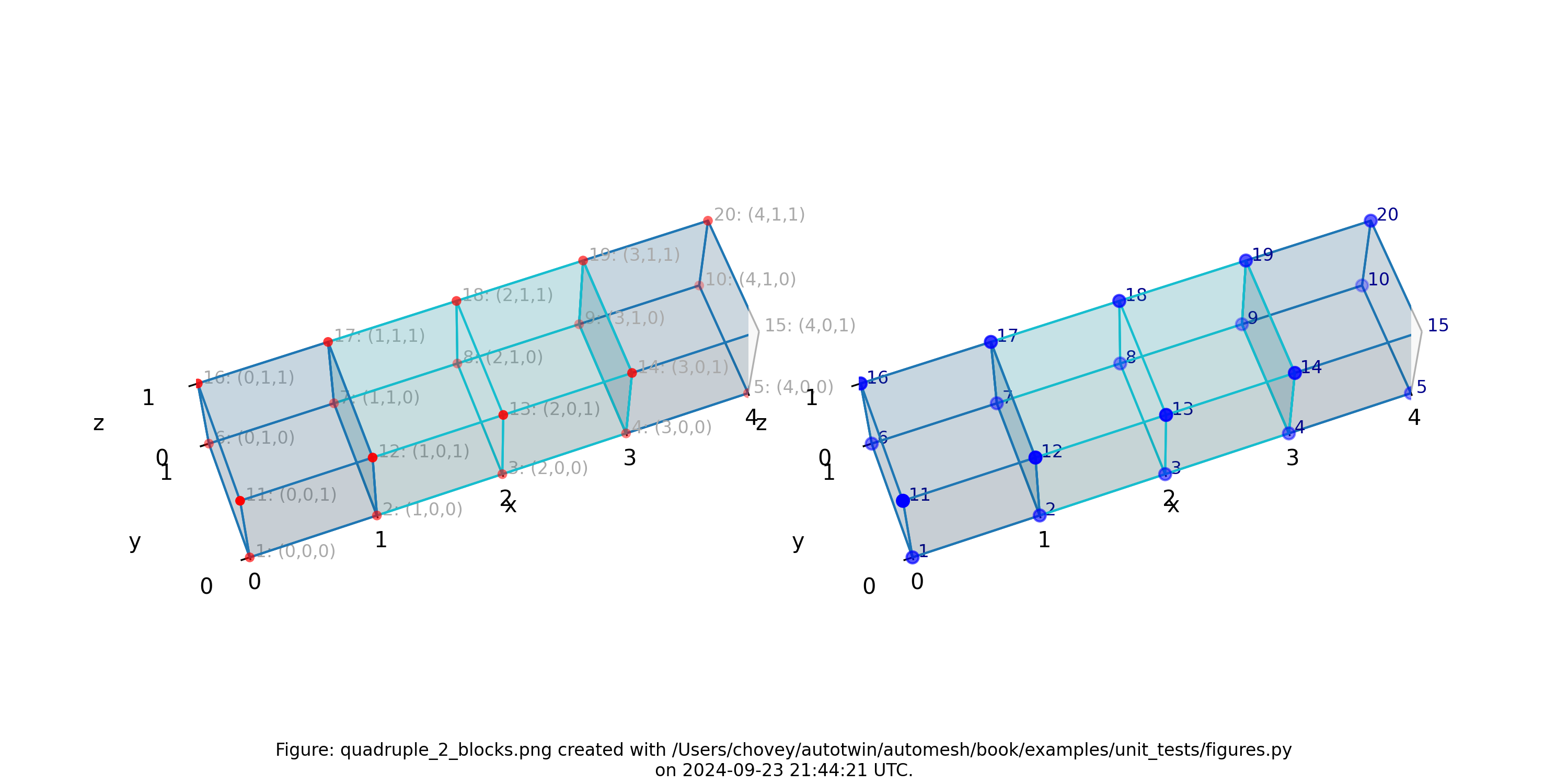
Figure 4.1-7: Mesh composed of two blocks with two elements elements each,
propagating along the x-axis, (left) lattice node numbers, (right) mesh
node numbers.
Quadruple with Two Blocks and Void
The .spn segmentation
102  #  x:1  y:1  z:1
103  #    2    1    1
0    #    3    1    1
102  #    4    1    1
where the segmentation 102 and 103 denotes block 102 and 103,
respectively, in the finite element mesh, and segmentation 0 is excluded from the mesh.
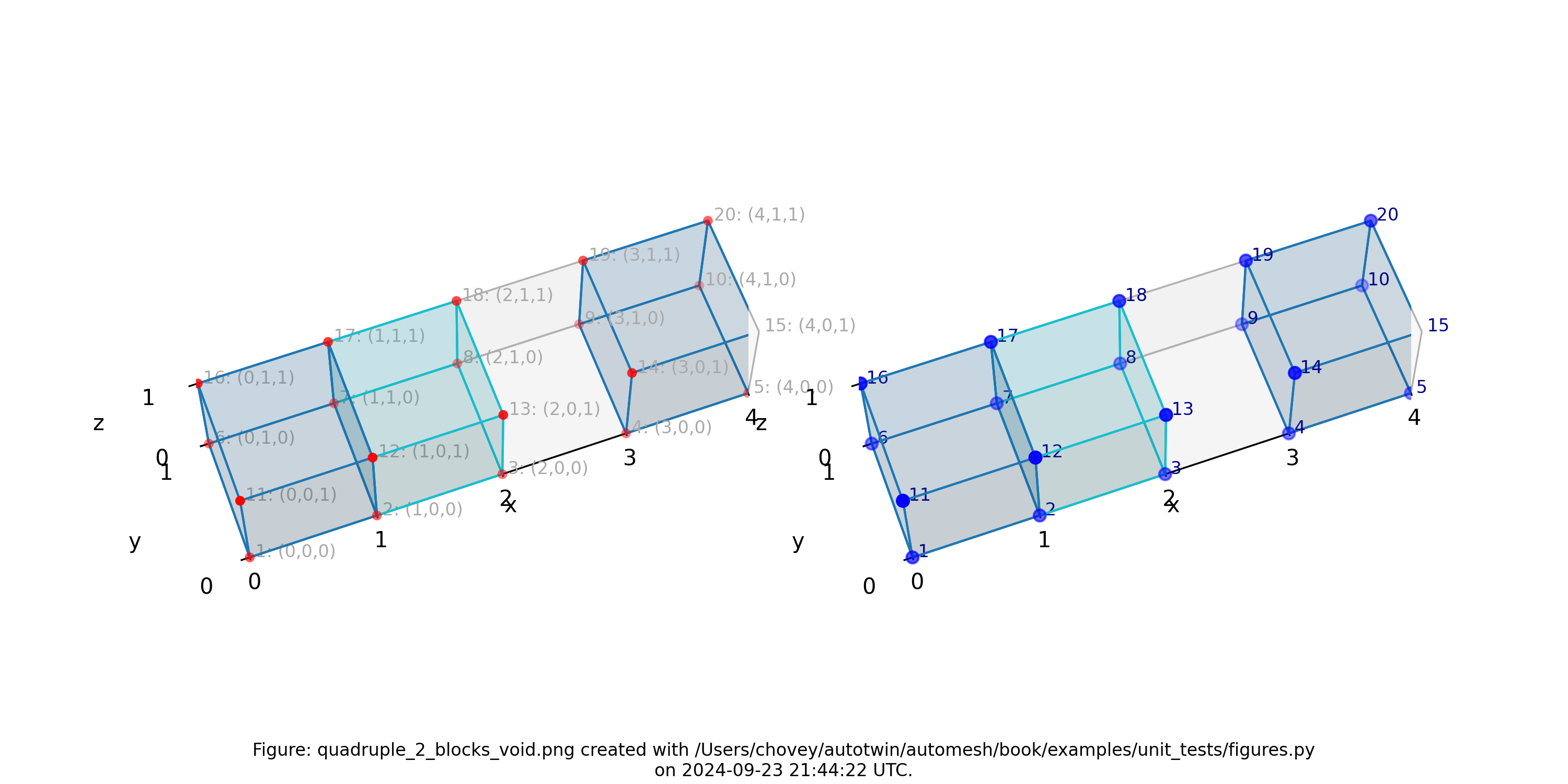
Figure 4.1-8: Mesh composed of one block with two elements, a second block with one
element, and a void, propagating along the x-axis, (left) lattice node
numbers, (right) mesh node numbers.
Cube
The .spn segmentation
11   #  x:1  y:1  z:1
11   #  _ 2  _ 1    1
11   #    1    2    1
11   #  _ 2  _ 2  _ 1
11   #    1    1    2
11   #  _ 2  _ 1    2
11   #    1    2    2
11   #  _ 2  _ 2  _ 2
where the segmentation 11 denotes block 11 in the finite element mesh.
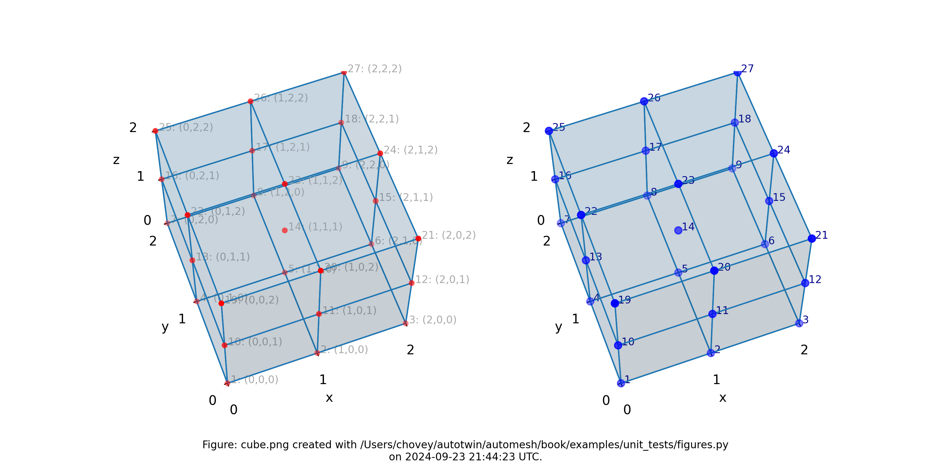
Figure 4.1-9: Mesh composed of one block with eight elements, (left) lattice node numbers, (right) mesh node numbers.
Cube with Multi Blocks and Void
The .spn segmentation
82   #  x:1  y:1  z:1
2    #  _ 2  _ 1    1
2    #    1    2    1
2    #  _ 2  _ 2  _ 1
0    #    1    1    2
31   #  _ 2  _ 1    2
0    #    1    2    2
44   #  _ 2  _ 2  _ 2
where the segmentation 82, 2, 31 and 44 denotes block 82, 2, 31
and 44, respectively, in the finite element mesh, and segmentation 0 will
be included from the finite element mesh.
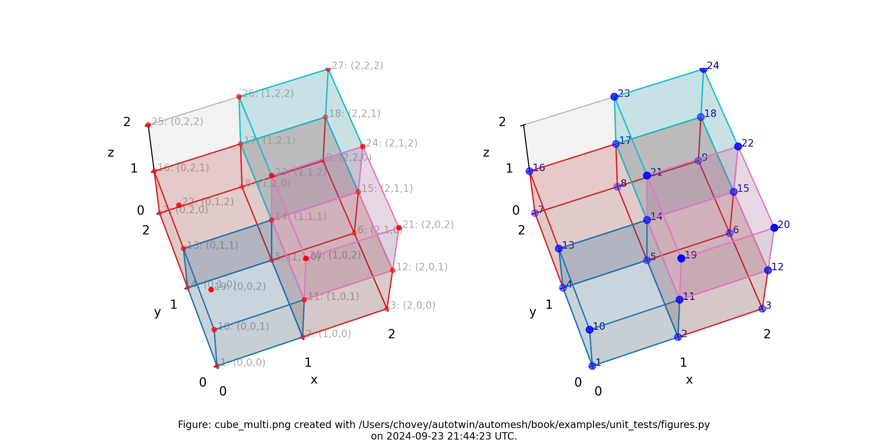
Figure 4.1-10: Mesh composed of four blocks (block 82 has one element, block 2
has three elements, block 31 has one element, and block 44 has one
element), (left) lattice node numbers, (right) mesh node numbers.
Cube with Inclusion
The .spn segmentation
11   #  x:1  y:1  z:1
11   #    2    1    1
11   #  _ 3  _ 1    1
11   #    1    2    1
11   #    2    2    1
11   #  _ 3  _ 2    1
11   #    1    3    1
11   #    2    3    1
11   #  _ 3  _ 3  _ 1
11   #    1    1    2
11   #    2    1    2
11   #  _ 3  _ 1    2
11   #    1    2    2
88   #    2    2    2
11   #  _ 3  _ 2    2
11   #    1    3    2
11   #    2    3    2
11   #  _ 3  _ 3  _ 2
11   #    1    1    3
11   #    2    1    3
11   #  _ 3  _ 1    3
11   #    1    2    3
11   #    2    2    3
11   #  _ 3  _ 2    3
11   #    1    3    3
11   #    2    3    3
11   #  _ 3  _ 3  _ 3
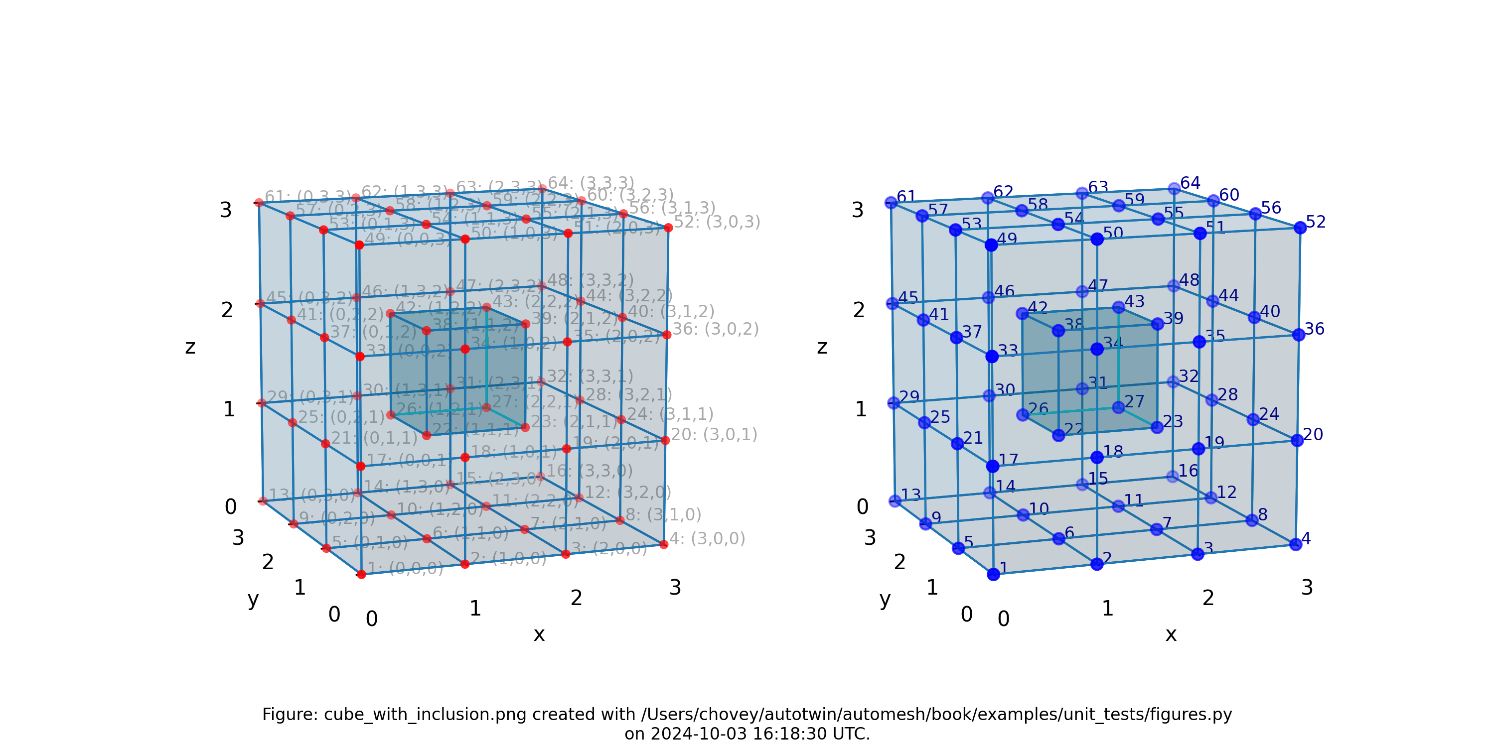
Figure 4.1-11: Mesh composed of 26 voxels of (block 11) and one voxel inslusion
(block 88), (left) lattice node numbers, (right) mesh node numbers.
Bracket
The .spn segmentation
1   #  x:1  y:1  z:1
1   #    2    1    1
1   #    3    1    1
1   #  _ 4  _ 1    1
1   #  x:1  y:2  z:1
1   #    2    2    1
1   #    3    2    1
1   #  _ 4  _ 2    1
1   #  x:1  y:3  z:1
1   #    2    3    1
0   #    3    3    1
0   #  _ 4  _ 3    1
1   #  x:1  y:4  z:1
1   #    2    4    1
0   #    3    4    1
0   #  _ 4  _ 4    1
where the segmentation 1 denotes block 1 in the finite element mesh,
and segmentation 0 is excluded from the mesh.
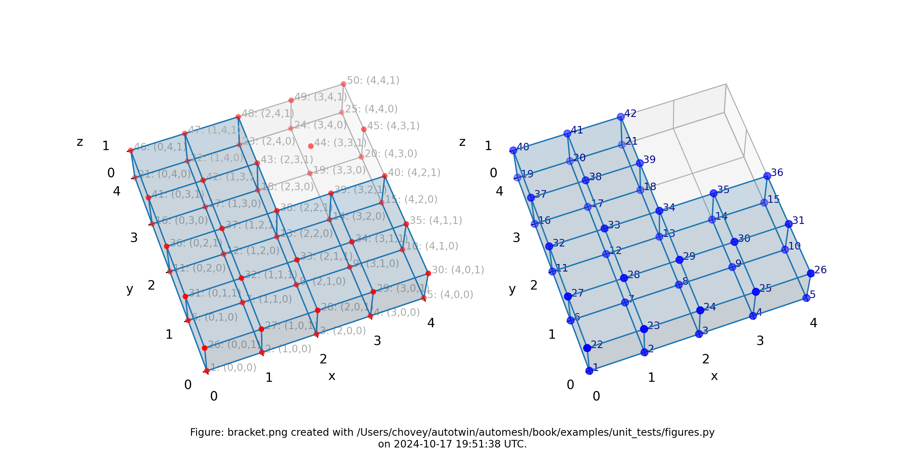
Figure 4.1-12: Mesh composed of a L-shaped bracket in the xy plane.
Letter F
The .spn segmentation
11   #  x:1  y:1  z:1
0    #    2    1    1
0    #  _ 3  _ 1    1
11   #    1    2    1
0    #    2    2    1
0    #  _ 3  _ 2    1
11   #    1    3    1
11   #    2    3    1
0    #  _ 3  _ 3    1
11   #    1    4    1
0    #    2    4    1
0    #  _ 3  _ 4    1
11   #    1    5    1
11   #    2    5    1
11   #  _ 3  _ 5  _ 1
where the segmentation 11 denotes block 11 in the finite element mesh.
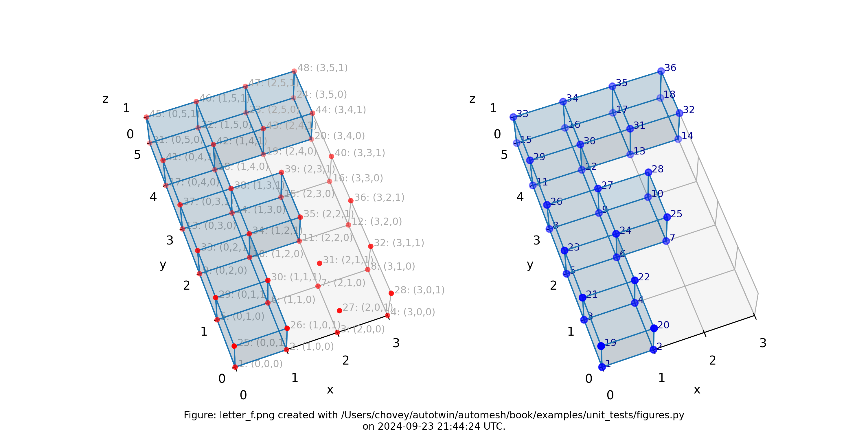
Figure 4.1-13: Mesh composed of a single block with eight elements, (left) lattice node numbers, (right) mesh node numbers.
Letter F in 3D
The .spn segmentation
1    #  x:1  y:1  z:1
1    #    2    1    1
1    #    3    1    1
1    #  _ 4  _ 1    1
1    #    1    2    1
1    #    2    2    1
1    #    3    2    1
1    #  _ 4  _ 2    1
1    #    1    3    1
1    #    2    3    1
1    #    3    3    1
1    #  _ 4  _ 3    1
1    #    1    4    1
1    #    2    4    1
1    #    3    4    1
1    #  _ 4  _ 4    1
1    #    1    5    1
1    #    2    5    1
1    #    3    5    1
1    #  _ 4  _ 5  _ 1
1    #  x:1  y:1  z:2
0    #    2    1    2
0    #    3    1    2
0    #  _ 4  _ 1    2
1    #    1    2    2
0    #    2    2    2
0    #    3    2    2
0    #  _ 4  _ 2    2
1    #    1    3    2
1    #    2    3    2
1    #    3    3    2
1    #  _ 4  _ 3    2
1    #    1    4    2
0    #    2    4    2
0    #    3    4    2
0    #  _ 4  _ 4    2
1    #    1    5    2
1    #    2    5    2
1    #    3    5    2
1    #  _ 4  _ 5  _ 2
1    #  x:1  y:1  z:3
0    #    2    1    j
0    #    3    1    2
0    #  _ 4  _ 1    2
1    #    1    2    3
0    #    2    2    3
0    #    3    2    3
0    #  _ 4  _ 2    3
1    #    1    3    3
0    #    2    3    3
0    #    3    3    3
0    #  _ 4  _ 3    3
1    #    1    4    3
0    #    2    4    3
0    #    3    4    3
0    #  _ 4  _ 4    3
1    #    1    5    3
1    #    2    5    3
1    #    3    5    3
1    #  _ 4  _ 5  _ 3
which corresponds to --nelx 4, --nely 5, and --nelz 3 in the
command line interface.
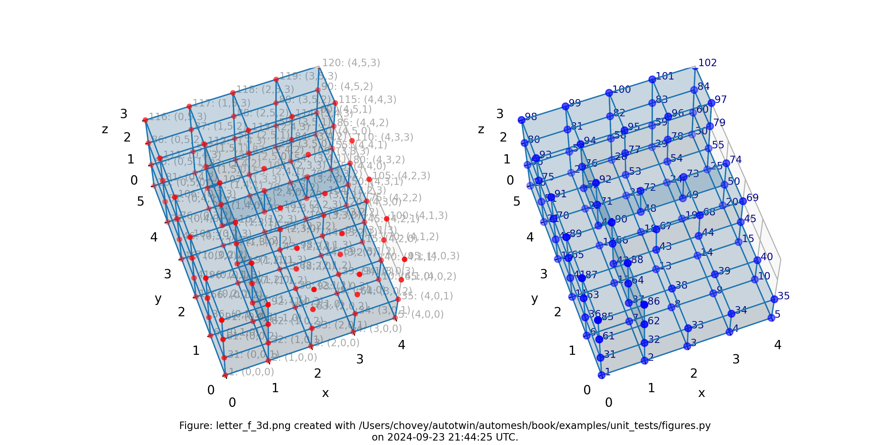
Figure 4.1-14: Mesh composed of a single block with thirty-nine elements, (left) lattice node numbers, (right) mesh node numbers.
The shape of the solid segmentation is more easily seen without the lattice and element nodes, and with decreased opacity, as shown below:
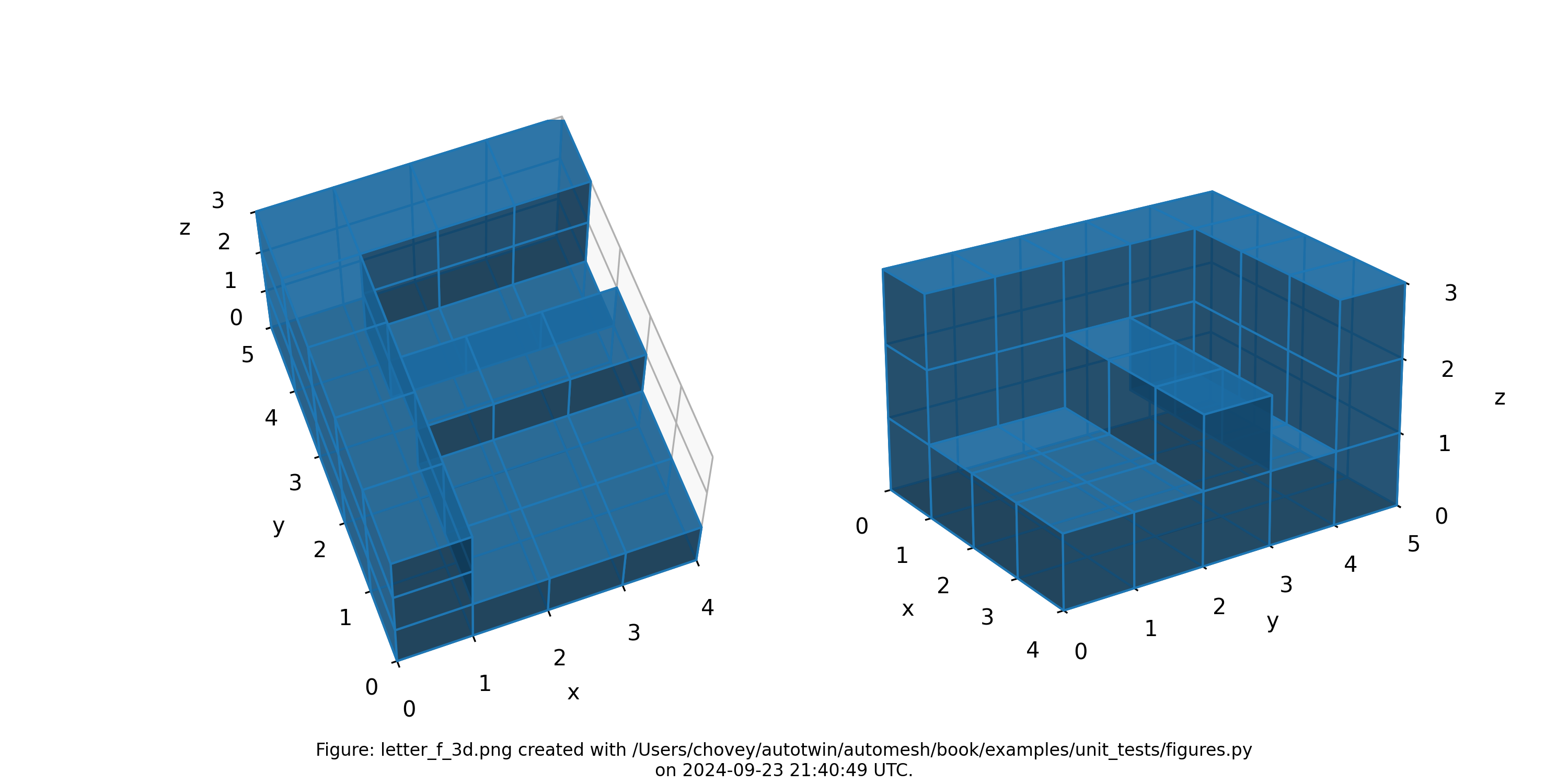
Figure 4.1-15: Mesh composed of a single block with thirty-nine elements, shown with decreased opacity and without lattice and element node numbers.
Sparse
The .spn segmentation
0    #  x:1  y:1  z:1
0    #    2    1    1
0    #    3    1    1
0    #    4    1    1
2    #  _ 5  _ 1    1
0    #    1    2    1
1    #    2    2    1
0    #    3    2    1
0    #    4    2    1
2    #  _ 5  _ 2    1
1    #    1    3    1
2    #    2    3    1
0    #    3    3    1
2    #    4    3    1
0    #  _ 5  _ 3    1
0    #    1    4    1
1    #    2    4    1
0    #    3    4    1
2    #    4    4    1
0    #  _ 5  _ 4    1
1    #    1    5    1
0    #    2    5    1
0    #    3    5    1
0    #    4    5    1
1    #  _ 5  _ 5  _ 1
2    #  x:1  y:1  z:2
0    #    2    1    2
2    #    3    1    2
0    #    4    1    2
0    #  _ 5  _ 1    2
1    #    1    2    2
1    #    2    2    2
0    #    3    2    2
2    #    4    2    2
2    #  _ 5  _ 2    2
2    #    1    3    2
0    #    2    3    2
0    #    3    3    2
0    #    4    3    2
0    #  _ 5  _ 3    2
1    #    1    4    2
0    #    2    4    2
0    #    3    4    2
2    #    4    4    2
0    #  _ 5  _ 4    2
2    #    1    5    2
0    #    2    5    2
2    #    3    5    2
0    #    4    5    2
2    #  _ 5  _ 5  _ 2
0    #  x:1  y:1  z:3
0    #    2    1    3
1    #    3    1    3
0    #    4    1    3
2    #  _ 5  _ 1    3
0    #    1    2    3
0    #    2    2    3
0    #    3    2    3
1    #    4    2    3
2    #  _ 5  _ 2    3
0    #    1    3    3
0    #    2    3    3
2    #    3    3    3
2    #    4    3    3
2    #  _ 5  _ 3    3
0    #    1    4    3
0    #    2    4    3
1    #    3    4    3
0    #    4    4    3
1    #  _ 5  _ 4    3
0    #    1    5    3
1    #    2    5    3
0    #    3    5    3
1    #    4    5    3
0    #  _ 5  _ 5  _ 3
0    #  x:1  y:1  z:4
1    #    2    1    4
2    #    3    1    4
1    #    4    1    4
2    #  _ 5  _ 1    4
2    #    1    2    4
0    #    2    2    4
2    #    3    2    4
0    #    4    2    4
1    #  _ 5  _ 2    4
1    #    1    3    4
2    #    2    3    4
2    #    3    3    4
0    #    4    3    4
0    #  _ 5  _ 3    4
2    #    1    4    4
1    #    2    4    4
1    #    3    4    4
1    #    4    4    4
1    #  _ 5  _ 4    4
0    #    1    5    4
0    #    2    5    4
1    #    3    5    4
0    #    4    5    4
0    #  _ 5  _ 5  _ 4
0    #  x:1  y:1  z:5
1    #    2    1    5
0    #    3    1    5
2    #    4    1    5
0    #  _ 5  _ 1    5
1    #    1    2    5
0    #    2    2    5
0    #    3    2    5
0    #    4    2    5
2    #  _ 5  _ 2    5
0    #    1    3    5
1    #    2    3    5
0    #    3    3    5
0    #    4    3    5
0    #  _ 5  _ 3    5
1    #    1    4    5
0    #    2    4    5
0    #    3    4    5
0    #    4    4    5
0    #  _ 5  _ 4    5
0    #    1    5    5
0    #    2    5    5
1    #    3    5    5
2    #    4    5    5
1    #  _ 5  _ 5  _ 5
where the segmentation 1 denotes block 1 and segmentation 2 denotes block 2 in the finite eelement mesh (with segmentation 0 excluded).
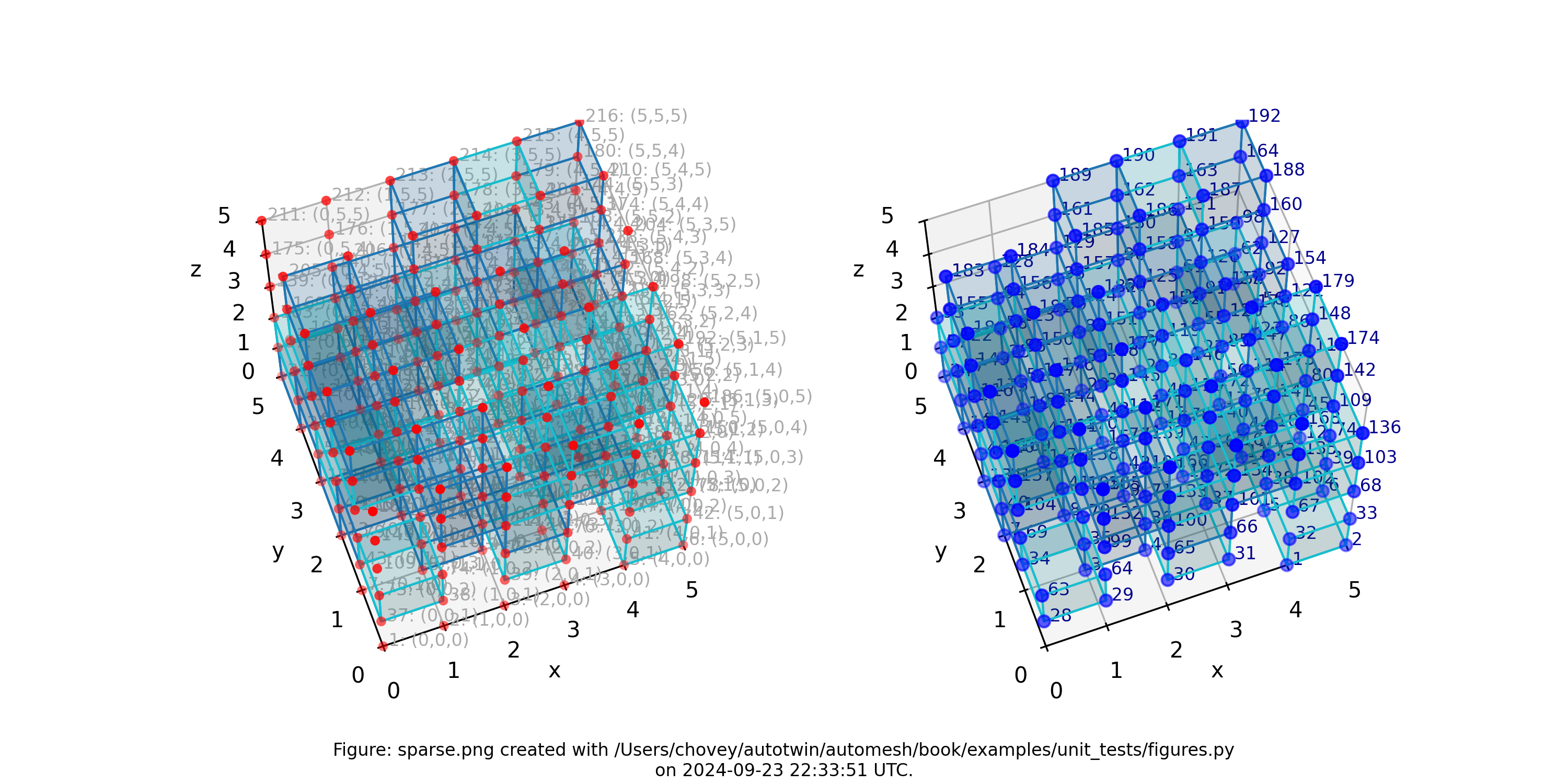
Figure 4.1-16: Sparse mesh composed of two materials at random voxel locations.
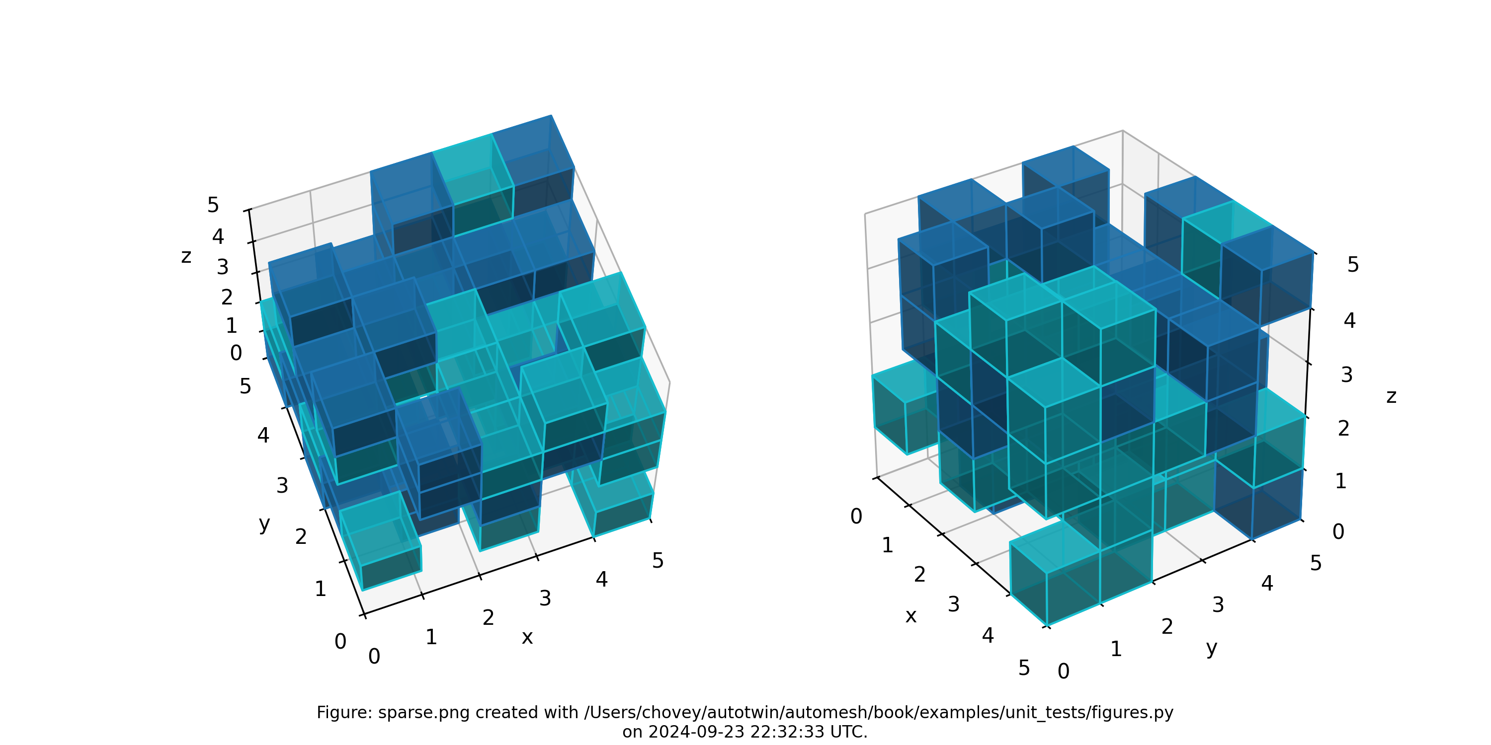
Figure 4.1-17: Sparse mesh composed of two materials at random voxel locations, shown with decreased opactity and without lattice and element node numbers.
Source
The figures were created with the following Python files:
examples_data.py
examples_data.py
r"""This module, examples_data.py, contains the data for
the unit test examples.
"""
from typing import Final
import numpy as np
import examples_types as ty
# Type aliases
Example = ty.Example
COMMON_TITLE: Final[str] = "Lattice Index and Coordinates: "
class Single(Example):
"""A specific example of a single voxel."""
figure_title: str = COMMON_TITLE + "Single"
file_stem: str = "single"
segmentation = np.array(
[
[
[
11,
],
],
],
dtype=np.uint8,
)
included_ids = (11,)
gold_lattice = ((1, 2, 4, 3, 5, 6, 8, 7),)
gold_mesh_lattice_connectivity = (
(
11,
(1, 2, 4, 3, 5, 6, 8, 7),
),
)
gold_mesh_element_connectivity = (
(
11,
(1, 2, 4, 3, 5, 6, 8, 7),
),
)
class DoubleX(Example):
"""A specific example of a double voxel, coursed along the x-axis."""
figure_title: str = COMMON_TITLE + "DoubleX"
file_stem: str = "double_x"
segmentation = np.array(
[
[
[
11,
11,
],
],
],
dtype=np.uint8,
)
included_ids = (11,)
gold_lattice = (
(1, 2, 5, 4, 7, 8, 11, 10),
(2, 3, 6, 5, 8, 9, 12, 11),
)
gold_mesh_lattice_connectivity = (
(
11,
(1, 2, 5, 4, 7, 8, 11, 10),
(2, 3, 6, 5, 8, 9, 12, 11),
),
)
gold_mesh_element_connectivity = (
(
11,
(1, 2, 5, 4, 7, 8, 11, 10),
(2, 3, 6, 5, 8, 9, 12, 11),
),
)
class DoubleY(Example):
"""A specific example of a double voxel, coursed along the y-axis."""
figure_title: str = COMMON_TITLE + "DoubleY"
file_stem: str = "double_y"
segmentation = np.array(
[
[
[
11,
],
[
11,
],
],
],
dtype=np.uint8,
)
included_ids = (11,)
gold_lattice = (
(1, 2, 4, 3, 7, 8, 10, 9),
(3, 4, 6, 5, 9, 10, 12, 11),
)
gold_mesh_lattice_connectivity = (
(
11,
(1, 2, 4, 3, 7, 8, 10, 9),
(3, 4, 6, 5, 9, 10, 12, 11),
),
)
gold_mesh_element_connectivity = (
(
11,
(1, 2, 4, 3, 7, 8, 10, 9),
(3, 4, 6, 5, 9, 10, 12, 11),
),
)
class TripleX(Example):
"""A triple voxel lattice, coursed along the x-axis."""
figure_title: str = COMMON_TITLE + "Triple"
file_stem: str = "triple_x"
segmentation = np.array(
[
[
[
11,
11,
11,
],
],
],
dtype=np.uint8,
)
included_ids = (11,)
gold_lattice = (
(1, 2, 6, 5, 9, 10, 14, 13),
(2, 3, 7, 6, 10, 11, 15, 14),
(3, 4, 8, 7, 11, 12, 16, 15),
)
gold_mesh_lattice_connectivity = (
(
11,
(1, 2, 6, 5, 9, 10, 14, 13),
(2, 3, 7, 6, 10, 11, 15, 14),
(3, 4, 8, 7, 11, 12, 16, 15),
),
)
gold_mesh_element_connectivity = (
(
11,
(1, 2, 6, 5, 9, 10, 14, 13),
(2, 3, 7, 6, 10, 11, 15, 14),
(3, 4, 8, 7, 11, 12, 16, 15),
),
)
class QuadrupleX(Example):
"""A quadruple voxel lattice, coursed along the x-axis."""
figure_title: str = COMMON_TITLE + "Quadruple"
file_stem: str = "quadruple_x"
segmentation = np.array(
[
[
[
11,
11,
11,
11,
],
],
],
dtype=np.uint8,
)
included_ids = (11,)
gold_lattice = (
(1, 2, 7, 6, 11, 12, 17, 16),
(2, 3, 8, 7, 12, 13, 18, 17),
(3, 4, 9, 8, 13, 14, 19, 18),
(4, 5, 10, 9, 14, 15, 20, 19),
)
gold_mesh_lattice_connectivity = (
(
11,
(1, 2, 7, 6, 11, 12, 17, 16),
(2, 3, 8, 7, 12, 13, 18, 17),
(3, 4, 9, 8, 13, 14, 19, 18),
(4, 5, 10, 9, 14, 15, 20, 19),
),
)
gold_mesh_element_connectivity = (
(
11,
(1, 2, 7, 6, 11, 12, 17, 16),
(2, 3, 8, 7, 12, 13, 18, 17),
(3, 4, 9, 8, 13, 14, 19, 18),
(4, 5, 10, 9, 14, 15, 20, 19),
),
)
class Quadruple2VoidsX(Example):
"""A quadruple voxel lattice, coursed along the x-axis, with two
intermediate voxels in the segmentation being void.
"""
figure_title: str = COMMON_TITLE + "Quadruple2VoidsX"
file_stem: str = "quadruple_2_voids_x"
segmentation = np.array(
[
[
[
99,
0,
0,
99,
],
],
],
dtype=np.uint8,
)
included_ids = (99,)
gold_lattice = (
(1, 2, 7, 6, 11, 12, 17, 16),
(2, 3, 8, 7, 12, 13, 18, 17),
(3, 4, 9, 8, 13, 14, 19, 18),
(4, 5, 10, 9, 14, 15, 20, 19),
)
gold_mesh_lattice_connectivity = (
(
99,
(1, 2, 7, 6, 11, 12, 17, 16),
(4, 5, 10, 9, 14, 15, 20, 19),
),
)
gold_mesh_element_connectivity = (
(
99,
(1, 2, 6, 5, 9, 10, 14, 13),
(3, 4, 8, 7, 11, 12, 16, 15),
),
)
class Quadruple2Blocks(Example):
"""A quadruple voxel lattice, with the first intermediate voxel being
the second block and the second intermediate voxel being void.
"""
figure_title: str = COMMON_TITLE + "Quadruple2Blocks"
file_stem: str = "quadruple_2_blocks"
segmentation = np.array(
[
[
[
100,
101,
101,
100,
],
],
],
dtype=np.uint8,
)
included_ids = (
100,
101,
)
gold_lattice = (
(1, 2, 7, 6, 11, 12, 17, 16),
(2, 3, 8, 7, 12, 13, 18, 17),
(3, 4, 9, 8, 13, 14, 19, 18),
(4, 5, 10, 9, 14, 15, 20, 19),
)
gold_mesh_lattice_connectivity = (
(
100,
(1, 2, 7, 6, 11, 12, 17, 16),
(4, 5, 10, 9, 14, 15, 20, 19),
),
(
101,
(2, 3, 8, 7, 12, 13, 18, 17),
(3, 4, 9, 8, 13, 14, 19, 18),
),
)
gold_mesh_element_connectivity = (
(
100,
(1, 2, 7, 6, 11, 12, 17, 16),
(4, 5, 10, 9, 14, 15, 20, 19),
),
(
101,
(2, 3, 8, 7, 12, 13, 18, 17),
(3, 4, 9, 8, 13, 14, 19, 18),
),
)
class Quadruple2BlocksVoid(Example):
"""A quadruple voxel lattice, with the first intermediate voxel being
the second block and the second intermediate voxel being void.
"""
figure_title: str = COMMON_TITLE + "Quadruple2BlocksVoid"
file_stem: str = "quadruple_2_blocks_void"
segmentation = np.array(
[
[
[
102,
103,
0,
102,
],
],
],
dtype=np.uint8,
)
included_ids = (
102,
103,
)
gold_lattice = (
(1, 2, 7, 6, 11, 12, 17, 16),
(2, 3, 8, 7, 12, 13, 18, 17),
(3, 4, 9, 8, 13, 14, 19, 18),
(4, 5, 10, 9, 14, 15, 20, 19),
)
gold_mesh_lattice_connectivity = (
(
102,
(1, 2, 7, 6, 11, 12, 17, 16),
(4, 5, 10, 9, 14, 15, 20, 19),
),
(
103,
(2, 3, 8, 7, 12, 13, 18, 17),
),
)
gold_mesh_element_connectivity = (
(
102,
(1, 2, 7, 6, 11, 12, 17, 16),
(4, 5, 10, 9, 14, 15, 20, 19),
),
(
103,
(2, 3, 8, 7, 12, 13, 18, 17),
),
)
class Cube(Example):
"""A (2 x 2 x 2) voxel cube."""
figure_title: str = COMMON_TITLE + "Cube"
file_stem: str = "cube"
segmentation = np.array(
[
[
[
11,
11,
],
[
11,
11,
],
],
[
[
11,
11,
],
[
11,
11,
],
],
],
dtype=np.uint8,
)
included_ids = (11,)
gold_lattice = (
(1, 2, 5, 4, 10, 11, 14, 13),
(2, 3, 6, 5, 11, 12, 15, 14),
(4, 5, 8, 7, 13, 14, 17, 16),
(5, 6, 9, 8, 14, 15, 18, 17),
(10, 11, 14, 13, 19, 20, 23, 22),
(11, 12, 15, 14, 20, 21, 24, 23),
(13, 14, 17, 16, 22, 23, 26, 25),
(14, 15, 18, 17, 23, 24, 27, 26),
)
gold_mesh_lattice_connectivity = (
(
11,
(1, 2, 5, 4, 10, 11, 14, 13),
(2, 3, 6, 5, 11, 12, 15, 14),
(4, 5, 8, 7, 13, 14, 17, 16),
(5, 6, 9, 8, 14, 15, 18, 17),
(10, 11, 14, 13, 19, 20, 23, 22),
(11, 12, 15, 14, 20, 21, 24, 23),
(13, 14, 17, 16, 22, 23, 26, 25),
(14, 15, 18, 17, 23, 24, 27, 26),
),
)
gold_mesh_element_connectivity = (
(
11,
(1, 2, 5, 4, 10, 11, 14, 13),
(2, 3, 6, 5, 11, 12, 15, 14),
(4, 5, 8, 7, 13, 14, 17, 16),
(5, 6, 9, 8, 14, 15, 18, 17),
(10, 11, 14, 13, 19, 20, 23, 22),
(11, 12, 15, 14, 20, 21, 24, 23),
(13, 14, 17, 16, 22, 23, 26, 25),
(14, 15, 18, 17, 23, 24, 27, 26),
),
)
class CubeMulti(Example):
"""A (2 x 2 x 2) voxel cube with two voids and six elements."""
figure_title: str = COMMON_TITLE + "CubeMulti"
file_stem: str = "cube_multi"
segmentation = np.array(
[
[
[
82,
2,
],
[
2,
2,
],
],
[
[
0,
31,
],
[
0,
44,
],
],
],
dtype=np.uint8,
)
included_ids = (
82,
2,
31,
44,
)
gold_lattice = (
(1, 2, 5, 4, 10, 11, 14, 13),
(2, 3, 6, 5, 11, 12, 15, 14),
(4, 5, 8, 7, 13, 14, 17, 16),
(5, 6, 9, 8, 14, 15, 18, 17),
(10, 11, 14, 13, 19, 20, 23, 22),
(11, 12, 15, 14, 20, 21, 24, 23),
(13, 14, 17, 16, 22, 23, 26, 25),
(14, 15, 18, 17, 23, 24, 27, 26),
)
gold_mesh_lattice_connectivity = (
# (
# 0,
# (10, 11, 14, 13, 19, 20, 23, 22),
# ),
# (
# 0,
# (13, 14, 17, 16, 22, 23, 26, 25),
(
2,
(2, 3, 6, 5, 11, 12, 15, 14),
(4, 5, 8, 7, 13, 14, 17, 16),
(5, 6, 9, 8, 14, 15, 18, 17),
),
(
31,
(11, 12, 15, 14, 20, 21, 24, 23),
),
(
44,
(14, 15, 18, 17, 23, 24, 27, 26),
),
(
82,
(1, 2, 5, 4, 10, 11, 14, 13),
),
)
gold_mesh_element_connectivity = (
(
2,
(2, 3, 6, 5, 11, 12, 15, 14),
(4, 5, 8, 7, 13, 14, 17, 16),
(5, 6, 9, 8, 14, 15, 18, 17),
),
(
31,
(11, 12, 15, 14, 19, 20, 22, 21),
),
(
44,
(14, 15, 18, 17, 21, 22, 24, 23),
),
(
82,
(1, 2, 5, 4, 10, 11, 14, 13),
),
)
class CubeWithInclusion(Example):
"""A (3 x 3 x 3) voxel cube with a single voxel inclusion
at the center.
"""
figure_title: str = COMMON_TITLE + "CubeWithInclusion"
file_stem: str = "cube_with_inclusion"
segmentation = np.array(
[
[
[
11,
11,
11,
],
[
11,
11,
11,
],
[
11,
11,
11,
],
],
[
[
11,
11,
11,
],
[
11,
88,
11,
],
[
11,
11,
11,
],
],
[
[
11,
11,
11,
],
[
11,
11,
11,
],
[
11,
11,
11,
],
],
],
dtype=np.uint8,
)
included_ids = (
11,
88,
)
gold_lattice = (
(1, 2, 6, 5, 17, 18, 22, 21),
(2, 3, 7, 6, 18, 19, 23, 22),
(3, 4, 8, 7, 19, 20, 24, 23),
(5, 6, 10, 9, 21, 22, 26, 25),
(6, 7, 11, 10, 22, 23, 27, 26),
(7, 8, 12, 11, 23, 24, 28, 27),
(9, 10, 14, 13, 25, 26, 30, 29),
(10, 11, 15, 14, 26, 27, 31, 30),
(11, 12, 16, 15, 27, 28, 32, 31),
(17, 18, 22, 21, 33, 34, 38, 37),
(18, 19, 23, 22, 34, 35, 39, 38),
(19, 20, 24, 23, 35, 36, 40, 39),
(21, 22, 26, 25, 37, 38, 42, 41),
(22, 23, 27, 26, 38, 39, 43, 42),
(23, 24, 28, 27, 39, 40, 44, 43),
(25, 26, 30, 29, 41, 42, 46, 45),
(26, 27, 31, 30, 42, 43, 47, 46),
(27, 28, 32, 31, 43, 44, 48, 47),
(33, 34, 38, 37, 49, 50, 54, 53),
(34, 35, 39, 38, 50, 51, 55, 54),
(35, 36, 40, 39, 51, 52, 56, 55),
(37, 38, 42, 41, 53, 54, 58, 57),
(38, 39, 43, 42, 54, 55, 59, 58),
(39, 40, 44, 43, 55, 56, 60, 59),
(41, 42, 46, 45, 57, 58, 62, 61),
(42, 43, 47, 46, 58, 59, 63, 62),
(43, 44, 48, 47, 59, 60, 64, 63),
)
gold_mesh_lattice_connectivity = (
(
11,
(1, 2, 6, 5, 17, 18, 22, 21),
(2, 3, 7, 6, 18, 19, 23, 22),
(3, 4, 8, 7, 19, 20, 24, 23),
(5, 6, 10, 9, 21, 22, 26, 25),
(6, 7, 11, 10, 22, 23, 27, 26),
(7, 8, 12, 11, 23, 24, 28, 27),
(9, 10, 14, 13, 25, 26, 30, 29),
(10, 11, 15, 14, 26, 27, 31, 30),
(11, 12, 16, 15, 27, 28, 32, 31),
(17, 18, 22, 21, 33, 34, 38, 37),
(18, 19, 23, 22, 34, 35, 39, 38),
(19, 20, 24, 23, 35, 36, 40, 39),
(21, 22, 26, 25, 37, 38, 42, 41),
(23, 24, 28, 27, 39, 40, 44, 43),
(25, 26, 30, 29, 41, 42, 46, 45),
(26, 27, 31, 30, 42, 43, 47, 46),
(27, 28, 32, 31, 43, 44, 48, 47),
(33, 34, 38, 37, 49, 50, 54, 53),
(34, 35, 39, 38, 50, 51, 55, 54),
(35, 36, 40, 39, 51, 52, 56, 55),
(37, 38, 42, 41, 53, 54, 58, 57),
(38, 39, 43, 42, 54, 55, 59, 58),
(39, 40, 44, 43, 55, 56, 60, 59),
(41, 42, 46, 45, 57, 58, 62, 61),
(42, 43, 47, 46, 58, 59, 63, 62),
(43, 44, 48, 47, 59, 60, 64, 63),
),
(
88,
(22, 23, 27, 26, 38, 39, 43, 42),
),
)
gold_mesh_element_connectivity = (
(
11,
(1, 2, 6, 5, 17, 18, 22, 21),
(2, 3, 7, 6, 18, 19, 23, 22),
(3, 4, 8, 7, 19, 20, 24, 23),
(5, 6, 10, 9, 21, 22, 26, 25),
(6, 7, 11, 10, 22, 23, 27, 26),
(7, 8, 12, 11, 23, 24, 28, 27),
(9, 10, 14, 13, 25, 26, 30, 29),
(10, 11, 15, 14, 26, 27, 31, 30),
(11, 12, 16, 15, 27, 28, 32, 31),
(17, 18, 22, 21, 33, 34, 38, 37),
(18, 19, 23, 22, 34, 35, 39, 38),
(19, 20, 24, 23, 35, 36, 40, 39),
(21, 22, 26, 25, 37, 38, 42, 41),
(23, 24, 28, 27, 39, 40, 44, 43),
(25, 26, 30, 29, 41, 42, 46, 45),
(26, 27, 31, 30, 42, 43, 47, 46),
(27, 28, 32, 31, 43, 44, 48, 47),
(33, 34, 38, 37, 49, 50, 54, 53),
(34, 35, 39, 38, 50, 51, 55, 54),
(35, 36, 40, 39, 51, 52, 56, 55),
(37, 38, 42, 41, 53, 54, 58, 57),
(38, 39, 43, 42, 54, 55, 59, 58),
(39, 40, 44, 43, 55, 56, 60, 59),
(41, 42, 46, 45, 57, 58, 62, 61),
(42, 43, 47, 46, 58, 59, 63, 62),
(43, 44, 48, 47, 59, 60, 64, 63),
),
(
88,
(22, 23, 27, 26, 38, 39, 43, 42),
),
)
class Bracket(Example):
"""An L-shape bracket in the xy plane."""
figure_title: str = COMMON_TITLE + "Bracket"
file_stem: str = "bracket"
segmentation = np.array(
[
[
[1, 1, 1, 1],
[1, 1, 1, 1],
[1, 1, 0, 0],
[1, 1, 0, 0],
],
]
)
included_ids = (1,)
gold_lattice = (
(1, 2, 7, 6, 26, 27, 32, 31),
(2, 3, 8, 7, 27, 28, 33, 32),
(3, 4, 9, 8, 28, 29, 34, 33),
(4, 5, 10, 9, 29, 30, 35, 34),
(6, 7, 12, 11, 31, 32, 37, 36),
(7, 8, 13, 12, 32, 33, 38, 37),
(8, 9, 14, 13, 33, 34, 39, 38),
(9, 10, 15, 14, 34, 35, 40, 39),
(11, 12, 17, 16, 36, 37, 42, 41),
(12, 13, 18, 17, 37, 38, 43, 42),
(13, 14, 19, 18, 38, 39, 44, 43),
(14, 15, 20, 19, 39, 40, 45, 44),
(16, 17, 22, 21, 41, 42, 47, 46),
(17, 18, 23, 22, 42, 43, 48, 47),
(18, 19, 24, 23, 43, 44, 49, 48),
(19, 20, 25, 24, 44, 45, 50, 49),
)
gold_mesh_lattice_connectivity = (
(
1,
(1, 2, 7, 6, 26, 27, 32, 31),
(2, 3, 8, 7, 27, 28, 33, 32),
(3, 4, 9, 8, 28, 29, 34, 33),
(4, 5, 10, 9, 29, 30, 35, 34),
(6, 7, 12, 11, 31, 32, 37, 36),
(7, 8, 13, 12, 32, 33, 38, 37),
(8, 9, 14, 13, 33, 34, 39, 38),
(9, 10, 15, 14, 34, 35, 40, 39),
(11, 12, 17, 16, 36, 37, 42, 41),
(12, 13, 18, 17, 37, 38, 43, 42),
(16, 17, 22, 21, 41, 42, 47, 46),
(17, 18, 23, 22, 42, 43, 48, 47),
),
)
gold_mesh_element_connectivity = (
(
1,
(1, 2, 7, 6, 22, 23, 28, 27),
(2, 3, 8, 7, 23, 24, 29, 28),
(3, 4, 9, 8, 24, 25, 30, 29),
(4, 5, 10, 9, 25, 26, 31, 30),
(6, 7, 12, 11, 27, 28, 33, 32),
(7, 8, 13, 12, 28, 29, 34, 33),
(8, 9, 14, 13, 29, 30, 35, 34),
(9, 10, 15, 14, 30, 31, 36, 35),
(11, 12, 17, 16, 32, 33, 38, 37),
(12, 13, 18, 17, 33, 34, 39, 38),
(16, 17, 20, 19, 37, 38, 41, 40),
(17, 18, 21, 20, 38, 39, 42, 41),
),
)
class LetterF(Example):
"""A minimal letter F example."""
figure_title: str = COMMON_TITLE + "LetterF"
file_stem: str = "letter_f"
segmentation = np.array(
[
[
[
11,
0,
0,
],
[
11,
0,
0,
],
[
11,
11,
0,
],
[
11,
0,
0,
],
[
11,
11,
11,
],
],
],
dtype=np.uint8,
)
included_ids = (11,)
gold_lattice = (
(1, 2, 6, 5, 25, 26, 30, 29),
(2, 3, 7, 6, 26, 27, 31, 30),
(3, 4, 8, 7, 27, 28, 32, 31),
(5, 6, 10, 9, 29, 30, 34, 33),
(6, 7, 11, 10, 30, 31, 35, 34),
(7, 8, 12, 11, 31, 32, 36, 35),
(9, 10, 14, 13, 33, 34, 38, 37),
(10, 11, 15, 14, 34, 35, 39, 38),
(11, 12, 16, 15, 35, 36, 40, 39),
(13, 14, 18, 17, 37, 38, 42, 41),
(14, 15, 19, 18, 38, 39, 43, 42),
(15, 16, 20, 19, 39, 40, 44, 43),
(17, 18, 22, 21, 41, 42, 46, 45),
(18, 19, 23, 22, 42, 43, 47, 46),
(19, 20, 24, 23, 43, 44, 48, 47),
)
gold_mesh_lattice_connectivity = (
(
11,
(1, 2, 6, 5, 25, 26, 30, 29),
# (2, 3, 7, 6, 26, 27, 31, 30),
# (3, 4, 8, 7, 27, 28, 32, 31),
(5, 6, 10, 9, 29, 30, 34, 33),
# (6, 7, 11, 10, 30, 31, 35, 34),
# (7, 8, 12, 11, 31, 32, 36, 35),
(9, 10, 14, 13, 33, 34, 38, 37),
(10, 11, 15, 14, 34, 35, 39, 38),
# (11, 12, 16, 15, 35, 36, 40, 39),
(13, 14, 18, 17, 37, 38, 42, 41),
# (14, 15, 19, 18, 38, 39, 43, 42),
# (15, 16, 20, 19, 39, 40, 44, 43),
(17, 18, 22, 21, 41, 42, 46, 45),
(18, 19, 23, 22, 42, 43, 47, 46),
(19, 20, 24, 23, 43, 44, 48, 47),
),
)
gold_mesh_element_connectivity = (
(
11,
(1, 2, 4, 3, 19, 20, 22, 21),
#
#
(3, 4, 6, 5, 21, 22, 24, 23),
#
#
(5, 6, 9, 8, 23, 24, 27, 26),
(6, 7, 10, 9, 24, 25, 28, 27),
#
(8, 9, 12, 11, 26, 27, 30, 29),
#
#
(11, 12, 16, 15, 29, 30, 34, 33),
(12, 13, 17, 16, 30, 31, 35, 34),
(13, 14, 18, 17, 31, 32, 36, 35),
),
)
class LetterF3D(Example):
"""A three dimensional variation of the letter F, in a non-standard
orientation.
"""
figure_title: str = COMMON_TITLE + "LetterF3D"
file_stem: str = "letter_f_3d"
segmentation = np.array(
[
[
[1, 1, 1, 1],
[1, 1, 1, 1],
[1, 1, 1, 1],
[1, 1, 1, 1],
[1, 1, 1, 1],
],
[
[1, 0, 0, 0],
[1, 0, 0, 0],
[1, 1, 1, 1],
[1, 0, 0, 0],
[1, 1, 1, 1],
],
[
[1, 0, 0, 0],
[1, 0, 0, 0],
[1, 0, 0, 0],
[1, 0, 0, 0],
[1, 1, 1, 1],
],
],
dtype=np.uint8,
)
included_ids = (1,)
gold_lattice = (
(1, 2, 7, 6, 31, 32, 37, 36),
(2, 3, 8, 7, 32, 33, 38, 37),
(3, 4, 9, 8, 33, 34, 39, 38),
(4, 5, 10, 9, 34, 35, 40, 39),
(6, 7, 12, 11, 36, 37, 42, 41),
(7, 8, 13, 12, 37, 38, 43, 42),
(8, 9, 14, 13, 38, 39, 44, 43),
(9, 10, 15, 14, 39, 40, 45, 44),
(11, 12, 17, 16, 41, 42, 47, 46),
(12, 13, 18, 17, 42, 43, 48, 47),
(13, 14, 19, 18, 43, 44, 49, 48),
(14, 15, 20, 19, 44, 45, 50, 49),
(16, 17, 22, 21, 46, 47, 52, 51),
(17, 18, 23, 22, 47, 48, 53, 52),
(18, 19, 24, 23, 48, 49, 54, 53),
(19, 20, 25, 24, 49, 50, 55, 54),
(21, 22, 27, 26, 51, 52, 57, 56),
(22, 23, 28, 27, 52, 53, 58, 57),
(23, 24, 29, 28, 53, 54, 59, 58),
(24, 25, 30, 29, 54, 55, 60, 59),
(31, 32, 37, 36, 61, 62, 67, 66),
(32, 33, 38, 37, 62, 63, 68, 67),
(33, 34, 39, 38, 63, 64, 69, 68),
(34, 35, 40, 39, 64, 65, 70, 69),
(36, 37, 42, 41, 66, 67, 72, 71),
(37, 38, 43, 42, 67, 68, 73, 72),
(38, 39, 44, 43, 68, 69, 74, 73),
(39, 40, 45, 44, 69, 70, 75, 74),
(41, 42, 47, 46, 71, 72, 77, 76),
(42, 43, 48, 47, 72, 73, 78, 77),
(43, 44, 49, 48, 73, 74, 79, 78),
(44, 45, 50, 49, 74, 75, 80, 79),
(46, 47, 52, 51, 76, 77, 82, 81),
(47, 48, 53, 52, 77, 78, 83, 82),
(48, 49, 54, 53, 78, 79, 84, 83),
(49, 50, 55, 54, 79, 80, 85, 84),
(51, 52, 57, 56, 81, 82, 87, 86),
(52, 53, 58, 57, 82, 83, 88, 87),
(53, 54, 59, 58, 83, 84, 89, 88),
(54, 55, 60, 59, 84, 85, 90, 89),
(61, 62, 67, 66, 91, 92, 97, 96),
(62, 63, 68, 67, 92, 93, 98, 97),
(63, 64, 69, 68, 93, 94, 99, 98),
(64, 65, 70, 69, 94, 95, 100, 99),
(66, 67, 72, 71, 96, 97, 102, 101),
(67, 68, 73, 72, 97, 98, 103, 102),
(68, 69, 74, 73, 98, 99, 104, 103),
(69, 70, 75, 74, 99, 100, 105, 104),
(71, 72, 77, 76, 101, 102, 107, 106),
(72, 73, 78, 77, 102, 103, 108, 107),
(73, 74, 79, 78, 103, 104, 109, 108),
(74, 75, 80, 79, 104, 105, 110, 109),
(76, 77, 82, 81, 106, 107, 112, 111),
(77, 78, 83, 82, 107, 108, 113, 112),
(78, 79, 84, 83, 108, 109, 114, 113),
(79, 80, 85, 84, 109, 110, 115, 114),
(81, 82, 87, 86, 111, 112, 117, 116),
(82, 83, 88, 87, 112, 113, 118, 117),
(83, 84, 89, 88, 113, 114, 119, 118),
(84, 85, 90, 89, 114, 115, 120, 119),
)
gold_mesh_lattice_connectivity = (
(
1,
(1, 2, 7, 6, 31, 32, 37, 36),
(2, 3, 8, 7, 32, 33, 38, 37),
(3, 4, 9, 8, 33, 34, 39, 38),
(4, 5, 10, 9, 34, 35, 40, 39),
(6, 7, 12, 11, 36, 37, 42, 41),
(7, 8, 13, 12, 37, 38, 43, 42),
(8, 9, 14, 13, 38, 39, 44, 43),
(9, 10, 15, 14, 39, 40, 45, 44),
(11, 12, 17, 16, 41, 42, 47, 46),
(12, 13, 18, 17, 42, 43, 48, 47),
(13, 14, 19, 18, 43, 44, 49, 48),
(14, 15, 20, 19, 44, 45, 50, 49),
(16, 17, 22, 21, 46, 47, 52, 51),
(17, 18, 23, 22, 47, 48, 53, 52),
(18, 19, 24, 23, 48, 49, 54, 53),
(19, 20, 25, 24, 49, 50, 55, 54),
(21, 22, 27, 26, 51, 52, 57, 56),
(22, 23, 28, 27, 52, 53, 58, 57),
(23, 24, 29, 28, 53, 54, 59, 58),
(24, 25, 30, 29, 54, 55, 60, 59),
(31, 32, 37, 36, 61, 62, 67, 66),
(36, 37, 42, 41, 66, 67, 72, 71),
(41, 42, 47, 46, 71, 72, 77, 76),
(42, 43, 48, 47, 72, 73, 78, 77),
(43, 44, 49, 48, 73, 74, 79, 78),
(44, 45, 50, 49, 74, 75, 80, 79),
(46, 47, 52, 51, 76, 77, 82, 81),
(51, 52, 57, 56, 81, 82, 87, 86),
(52, 53, 58, 57, 82, 83, 88, 87),
(53, 54, 59, 58, 83, 84, 89, 88),
(54, 55, 60, 59, 84, 85, 90, 89),
(61, 62, 67, 66, 91, 92, 97, 96),
(66, 67, 72, 71, 96, 97, 102, 101),
(71, 72, 77, 76, 101, 102, 107, 106),
(76, 77, 82, 81, 106, 107, 112, 111),
(81, 82, 87, 86, 111, 112, 117, 116),
(82, 83, 88, 87, 112, 113, 118, 117),
(83, 84, 89, 88, 113, 114, 119, 118),
(84, 85, 90, 89, 114, 115, 120, 119),
),
)
gold_mesh_element_connectivity = (
(
1,
(1, 2, 7, 6, 31, 32, 37, 36),
(2, 3, 8, 7, 32, 33, 38, 37),
(3, 4, 9, 8, 33, 34, 39, 38),
(4, 5, 10, 9, 34, 35, 40, 39),
(6, 7, 12, 11, 36, 37, 42, 41),
(7, 8, 13, 12, 37, 38, 43, 42),
(8, 9, 14, 13, 38, 39, 44, 43),
(9, 10, 15, 14, 39, 40, 45, 44),
(11, 12, 17, 16, 41, 42, 47, 46),
(12, 13, 18, 17, 42, 43, 48, 47),
(13, 14, 19, 18, 43, 44, 49, 48),
(14, 15, 20, 19, 44, 45, 50, 49),
(16, 17, 22, 21, 46, 47, 52, 51),
(17, 18, 23, 22, 47, 48, 53, 52),
(18, 19, 24, 23, 48, 49, 54, 53),
(19, 20, 25, 24, 49, 50, 55, 54),
(21, 22, 27, 26, 51, 52, 57, 56),
(22, 23, 28, 27, 52, 53, 58, 57),
(23, 24, 29, 28, 53, 54, 59, 58),
(24, 25, 30, 29, 54, 55, 60, 59),
(31, 32, 37, 36, 61, 62, 64, 63),
(36, 37, 42, 41, 63, 64, 66, 65),
(41, 42, 47, 46, 65, 66, 71, 70),
(42, 43, 48, 47, 66, 67, 72, 71),
(43, 44, 49, 48, 67, 68, 73, 72),
(44, 45, 50, 49, 68, 69, 74, 73),
(46, 47, 52, 51, 70, 71, 76, 75),
(51, 52, 57, 56, 75, 76, 81, 80),
(52, 53, 58, 57, 76, 77, 82, 81),
(53, 54, 59, 58, 77, 78, 83, 82),
(54, 55, 60, 59, 78, 79, 84, 83),
(61, 62, 64, 63, 85, 86, 88, 87),
(63, 64, 66, 65, 87, 88, 90, 89),
(65, 66, 71, 70, 89, 90, 92, 91),
(70, 71, 76, 75, 91, 92, 94, 93),
(75, 76, 81, 80, 93, 94, 99, 98),
(76, 77, 82, 81, 94, 95, 100, 99),
(77, 78, 83, 82, 95, 96, 101, 100),
(78, 79, 84, 83, 96, 97, 102, 101),
),
)
class Sparse(Example):
"""A randomized 5x5x5 segmentation."""
figure_title: str = COMMON_TITLE + "Sparse"
file_stem: str = "sparse"
segmentation = np.array(
[
[
[0, 0, 0, 0, 2],
[0, 1, 0, 0, 2],
[1, 2, 0, 2, 0],
[0, 1, 0, 2, 0],
[1, 0, 0, 0, 1],
],
[
[2, 0, 2, 0, 0],
[1, 1, 0, 2, 2],
[2, 0, 0, 0, 0],
[1, 0, 0, 2, 0],
[2, 0, 2, 0, 2],
],
[
[0, 0, 1, 0, 2],
[0, 0, 0, 1, 2],
[0, 0, 2, 2, 2],
[0, 0, 1, 0, 1],
[0, 1, 0, 1, 0],
],
[
[0, 1, 2, 1, 2],
[2, 0, 2, 0, 1],
[1, 2, 2, 0, 0],
[2, 1, 1, 1, 1],
[0, 0, 1, 0, 0],
],
[
[0, 1, 0, 2, 0],
[1, 0, 0, 0, 2],
[0, 1, 0, 0, 0],
[1, 0, 0, 0, 0],
[0, 0, 1, 2, 1],
],
],
dtype=np.uint8,
)
included_ids = (
1,
2,
)
gold_lattice = (
(1, 2, 8, 7, 37, 38, 44, 43),
(2, 3, 9, 8, 38, 39, 45, 44),
(3, 4, 10, 9, 39, 40, 46, 45),
(4, 5, 11, 10, 40, 41, 47, 46),
(5, 6, 12, 11, 41, 42, 48, 47),
(7, 8, 14, 13, 43, 44, 50, 49),
(8, 9, 15, 14, 44, 45, 51, 50),
(9, 10, 16, 15, 45, 46, 52, 51),
(10, 11, 17, 16, 46, 47, 53, 52),
(11, 12, 18, 17, 47, 48, 54, 53),
(13, 14, 20, 19, 49, 50, 56, 55),
(14, 15, 21, 20, 50, 51, 57, 56),
(15, 16, 22, 21, 51, 52, 58, 57),
(16, 17, 23, 22, 52, 53, 59, 58),
(17, 18, 24, 23, 53, 54, 60, 59),
(19, 20, 26, 25, 55, 56, 62, 61),
(20, 21, 27, 26, 56, 57, 63, 62),
(21, 22, 28, 27, 57, 58, 64, 63),
(22, 23, 29, 28, 58, 59, 65, 64),
(23, 24, 30, 29, 59, 60, 66, 65),
(25, 26, 32, 31, 61, 62, 68, 67),
(26, 27, 33, 32, 62, 63, 69, 68),
(27, 28, 34, 33, 63, 64, 70, 69),
(28, 29, 35, 34, 64, 65, 71, 70),
(29, 30, 36, 35, 65, 66, 72, 71),
(37, 38, 44, 43, 73, 74, 80, 79),
(38, 39, 45, 44, 74, 75, 81, 80),
(39, 40, 46, 45, 75, 76, 82, 81),
(40, 41, 47, 46, 76, 77, 83, 82),
(41, 42, 48, 47, 77, 78, 84, 83),
(43, 44, 50, 49, 79, 80, 86, 85),
(44, 45, 51, 50, 80, 81, 87, 86),
(45, 46, 52, 51, 81, 82, 88, 87),
(46, 47, 53, 52, 82, 83, 89, 88),
(47, 48, 54, 53, 83, 84, 90, 89),
(49, 50, 56, 55, 85, 86, 92, 91),
(50, 51, 57, 56, 86, 87, 93, 92),
(51, 52, 58, 57, 87, 88, 94, 93),
(52, 53, 59, 58, 88, 89, 95, 94),
(53, 54, 60, 59, 89, 90, 96, 95),
(55, 56, 62, 61, 91, 92, 98, 97),
(56, 57, 63, 62, 92, 93, 99, 98),
(57, 58, 64, 63, 93, 94, 100, 99),
(58, 59, 65, 64, 94, 95, 101, 100),
(59, 60, 66, 65, 95, 96, 102, 101),
(61, 62, 68, 67, 97, 98, 104, 103),
(62, 63, 69, 68, 98, 99, 105, 104),
(63, 64, 70, 69, 99, 100, 106, 105),
(64, 65, 71, 70, 100, 101, 107, 106),
(65, 66, 72, 71, 101, 102, 108, 107),
(73, 74, 80, 79, 109, 110, 116, 115),
(74, 75, 81, 80, 110, 111, 117, 116),
(75, 76, 82, 81, 111, 112, 118, 117),
(76, 77, 83, 82, 112, 113, 119, 118),
(77, 78, 84, 83, 113, 114, 120, 119),
(79, 80, 86, 85, 115, 116, 122, 121),
(80, 81, 87, 86, 116, 117, 123, 122),
(81, 82, 88, 87, 117, 118, 124, 123),
(82, 83, 89, 88, 118, 119, 125, 124),
(83, 84, 90, 89, 119, 120, 126, 125),
(85, 86, 92, 91, 121, 122, 128, 127),
(86, 87, 93, 92, 122, 123, 129, 128),
(87, 88, 94, 93, 123, 124, 130, 129),
(88, 89, 95, 94, 124, 125, 131, 130),
(89, 90, 96, 95, 125, 126, 132, 131),
(91, 92, 98, 97, 127, 128, 134, 133),
(92, 93, 99, 98, 128, 129, 135, 134),
(93, 94, 100, 99, 129, 130, 136, 135),
(94, 95, 101, 100, 130, 131, 137, 136),
(95, 96, 102, 101, 131, 132, 138, 137),
(97, 98, 104, 103, 133, 134, 140, 139),
(98, 99, 105, 104, 134, 135, 141, 140),
(99, 100, 106, 105, 135, 136, 142, 141),
(100, 101, 107, 106, 136, 137, 143, 142),
(101, 102, 108, 107, 137, 138, 144, 143),
(109, 110, 116, 115, 145, 146, 152, 151),
(110, 111, 117, 116, 146, 147, 153, 152),
(111, 112, 118, 117, 147, 148, 154, 153),
(112, 113, 119, 118, 148, 149, 155, 154),
(113, 114, 120, 119, 149, 150, 156, 155),
(115, 116, 122, 121, 151, 152, 158, 157),
(116, 117, 123, 122, 152, 153, 159, 158),
(117, 118, 124, 123, 153, 154, 160, 159),
(118, 119, 125, 124, 154, 155, 161, 160),
(119, 120, 126, 125, 155, 156, 162, 161),
(121, 122, 128, 127, 157, 158, 164, 163),
(122, 123, 129, 128, 158, 159, 165, 164),
(123, 124, 130, 129, 159, 160, 166, 165),
(124, 125, 131, 130, 160, 161, 167, 166),
(125, 126, 132, 131, 161, 162, 168, 167),
(127, 128, 134, 133, 163, 164, 170, 169),
(128, 129, 135, 134, 164, 165, 171, 170),
(129, 130, 136, 135, 165, 166, 172, 171),
(130, 131, 137, 136, 166, 167, 173, 172),
(131, 132, 138, 137, 167, 168, 174, 173),
(133, 134, 140, 139, 169, 170, 176, 175),
(134, 135, 141, 140, 170, 171, 177, 176),
(135, 136, 142, 141, 171, 172, 178, 177),
(136, 137, 143, 142, 172, 173, 179, 178),
(137, 138, 144, 143, 173, 174, 180, 179),
(145, 146, 152, 151, 181, 182, 188, 187),
(146, 147, 153, 152, 182, 183, 189, 188),
(147, 148, 154, 153, 183, 184, 190, 189),
(148, 149, 155, 154, 184, 185, 191, 190),
(149, 150, 156, 155, 185, 186, 192, 191),
(151, 152, 158, 157, 187, 188, 194, 193),
(152, 153, 159, 158, 188, 189, 195, 194),
(153, 154, 160, 159, 189, 190, 196, 195),
(154, 155, 161, 160, 190, 191, 197, 196),
(155, 156, 162, 161, 191, 192, 198, 197),
(157, 158, 164, 163, 193, 194, 200, 199),
(158, 159, 165, 164, 194, 195, 201, 200),
(159, 160, 166, 165, 195, 196, 202, 201),
(160, 161, 167, 166, 196, 197, 203, 202),
(161, 162, 168, 167, 197, 198, 204, 203),
(163, 164, 170, 169, 199, 200, 206, 205),
(164, 165, 171, 170, 200, 201, 207, 206),
(165, 166, 172, 171, 201, 202, 208, 207),
(166, 167, 173, 172, 202, 203, 209, 208),
(167, 168, 174, 173, 203, 204, 210, 209),
(169, 170, 176, 175, 205, 206, 212, 211),
(170, 171, 177, 176, 206, 207, 213, 212),
(171, 172, 178, 177, 207, 208, 214, 213),
(172, 173, 179, 178, 208, 209, 215, 214),
(173, 174, 180, 179, 209, 210, 216, 215),
)
gold_mesh_lattice_connectivity = (
(
1,
(8, 9, 15, 14, 44, 45, 51, 50),
(13, 14, 20, 19, 49, 50, 56, 55),
(20, 21, 27, 26, 56, 57, 63, 62),
(25, 26, 32, 31, 61, 62, 68, 67),
(29, 30, 36, 35, 65, 66, 72, 71),
(43, 44, 50, 49, 79, 80, 86, 85),
(44, 45, 51, 50, 80, 81, 87, 86),
(55, 56, 62, 61, 91, 92, 98, 97),
(75, 76, 82, 81, 111, 112, 118, 117),
(82, 83, 89, 88, 118, 119, 125, 124),
(93, 94, 100, 99, 129, 130, 136, 135),
(95, 96, 102, 101, 131, 132, 138, 137),
(98, 99, 105, 104, 134, 135, 141, 140),
(100, 101, 107, 106, 136, 137, 143, 142),
(110, 111, 117, 116, 146, 147, 153, 152),
(112, 113, 119, 118, 148, 149, 155, 154),
(119, 120, 126, 125, 155, 156, 162, 161),
(121, 122, 128, 127, 157, 158, 164, 163),
(128, 129, 135, 134, 164, 165, 171, 170),
(129, 130, 136, 135, 165, 166, 172, 171),
(130, 131, 137, 136, 166, 167, 173, 172),
(131, 132, 138, 137, 167, 168, 174, 173),
(135, 136, 142, 141, 171, 172, 178, 177),
(146, 147, 153, 152, 182, 183, 189, 188),
(151, 152, 158, 157, 187, 188, 194, 193),
(158, 159, 165, 164, 194, 195, 201, 200),
(163, 164, 170, 169, 199, 200, 206, 205),
(171, 172, 178, 177, 207, 208, 214, 213),
(173, 174, 180, 179, 209, 210, 216, 215),
),
(
2,
(5, 6, 12, 11, 41, 42, 48, 47),
(11, 12, 18, 17, 47, 48, 54, 53),
(14, 15, 21, 20, 50, 51, 57, 56),
(16, 17, 23, 22, 52, 53, 59, 58),
(22, 23, 29, 28, 58, 59, 65, 64),
(37, 38, 44, 43, 73, 74, 80, 79),
(39, 40, 46, 45, 75, 76, 82, 81),
(46, 47, 53, 52, 82, 83, 89, 88),
(47, 48, 54, 53, 83, 84, 90, 89),
(49, 50, 56, 55, 85, 86, 92, 91),
(58, 59, 65, 64, 94, 95, 101, 100),
(61, 62, 68, 67, 97, 98, 104, 103),
(63, 64, 70, 69, 99, 100, 106, 105),
(65, 66, 72, 71, 101, 102, 108, 107),
(77, 78, 84, 83, 113, 114, 120, 119),
(83, 84, 90, 89, 119, 120, 126, 125),
(87, 88, 94, 93, 123, 124, 130, 129),
(88, 89, 95, 94, 124, 125, 131, 130),
(89, 90, 96, 95, 125, 126, 132, 131),
(111, 112, 118, 117, 147, 148, 154, 153),
(113, 114, 120, 119, 149, 150, 156, 155),
(115, 116, 122, 121, 151, 152, 158, 157),
(117, 118, 124, 123, 153, 154, 160, 159),
(122, 123, 129, 128, 158, 159, 165, 164),
(123, 124, 130, 129, 159, 160, 166, 165),
(127, 128, 134, 133, 163, 164, 170, 169),
(148, 149, 155, 154, 184, 185, 191, 190),
(155, 156, 162, 161, 191, 192, 198, 197),
(172, 173, 179, 178, 208, 209, 215, 214),
),
)
gold_mesh_element_connectivity = (
(
1,
(3, 4, 9, 8, 35, 36, 42, 41),
(7, 8, 14, 13, 40, 41, 47, 46),
(14, 15, 20, 19, 47, 48, 53, 52),
(18, 19, 25, 24, 51, 52, 58, 57),
(22, 23, 27, 26, 55, 56, 62, 61),
(34, 35, 41, 40, 69, 70, 76, 75),
(35, 36, 42, 41, 70, 71, 77, 76),
(46, 47, 52, 51, 81, 82, 88, 87),
(65, 66, 72, 71, 100, 101, 107, 106),
(72, 73, 79, 78, 107, 108, 114, 113),
(83, 84, 90, 89, 118, 119, 125, 124),
(85, 86, 92, 91, 120, 121, 127, 126),
(88, 89, 95, 94, 123, 124, 129, 128),
(90, 91, 97, 96, 125, 126, 131, 130),
(99, 100, 106, 105, 132, 133, 139, 138),
(101, 102, 108, 107, 134, 135, 141, 140),
(108, 109, 115, 114, 141, 142, 148, 147),
(110, 111, 117, 116, 143, 144, 150, 149),
(117, 118, 124, 123, 150, 151, 157, 156),
(118, 119, 125, 124, 151, 152, 158, 157),
(119, 120, 126, 125, 152, 153, 159, 158),
(120, 121, 127, 126, 153, 154, 160, 159),
(124, 125, 130, 129, 157, 158, 162, 161),
(132, 133, 139, 138, 165, 166, 171, 170),
(137, 138, 144, 143, 169, 170, 176, 175),
(144, 145, 151, 150, 176, 177, 182, 181),
(149, 150, 156, 155, 180, 181, 184, 183),
(157, 158, 162, 161, 185, 186, 190, 189),
(159, 160, 164, 163, 187, 188, 192, 191),
),
(
2,
(1, 2, 6, 5, 32, 33, 39, 38),
(5, 6, 12, 11, 38, 39, 45, 44),
(8, 9, 15, 14, 41, 42, 48, 47),
(10, 11, 17, 16, 43, 44, 50, 49),
(16, 17, 22, 21, 49, 50, 55, 54),
(28, 29, 35, 34, 63, 64, 70, 69),
(30, 31, 37, 36, 65, 66, 72, 71),
(37, 38, 44, 43, 72, 73, 79, 78),
(38, 39, 45, 44, 73, 74, 80, 79),
(40, 41, 47, 46, 75, 76, 82, 81),
(49, 50, 55, 54, 84, 85, 91, 90),
(51, 52, 58, 57, 87, 88, 94, 93),
(53, 54, 60, 59, 89, 90, 96, 95),
(55, 56, 62, 61, 91, 92, 98, 97),
(67, 68, 74, 73, 102, 103, 109, 108),
(73, 74, 80, 79, 108, 109, 115, 114),
(77, 78, 84, 83, 112, 113, 119, 118),
(78, 79, 85, 84, 113, 114, 120, 119),
(79, 80, 86, 85, 114, 115, 121, 120),
(100, 101, 107, 106, 133, 134, 140, 139),
(102, 103, 109, 108, 135, 136, 142, 141),
(104, 105, 111, 110, 137, 138, 144, 143),
(106, 107, 113, 112, 139, 140, 146, 145),
(111, 112, 118, 117, 144, 145, 151, 150),
(112, 113, 119, 118, 145, 146, 152, 151),
(116, 117, 123, 122, 149, 150, 156, 155),
(134, 135, 141, 140, 167, 168, 173, 172),
(141, 142, 148, 147, 173, 174, 179, 178),
(158, 159, 163, 162, 186, 187, 191, 190),
),
)
examples_figures.py
examples_figures.py
r"""This module, examples_figures.py, demonstrates creating a pixel slice in
the (x, y) plane, and then appending layers in the z axis, to create a 3D
voxel lattice, as a precursor for a hexahedral finite element mesh.

Example
-------
source ~/autotwin/automesh/.venv/bin/activate
pip install matplotlib
cd ~/autotwin/automesh/book/examples/unit_tests
python examples_figures.py

Output
-----
The `output_npy` segmentation data files
The `output_png` visualization files
"""

# standard library
import datetime
from pathlib import Path
from typing import Final

# third-party library
import matplotlib.pyplot as plt
from matplotlib.colors import LightSource
import numpy as np
from numpy.typing import NDArray

import examples_types as types
import examples_data as data

# Type aliases
Example = types.Example


def lattice_connectivity(ex: Example) -> NDArray[np.uint8]:
    """Given an Example, prints the lattice connectivity."""
    offset = 0
    nz, ny, nx = ex.segmentation.shape
    nzp, nyp, nxp = nz + 1, ny + 1, nx + 1

    # Generate the lattice nodes
    lattice_nodes = []

    lattice_node = 0
    for k in range(nzp):
        for j in range(nyp):
            for i in range(nxp):
                lattice_node += 1
                lattice_nodes.append([lattice_node, i, j, k])

    # connectivity for each voxel
    cvs = []

    offset = 0

    # print("processing indices...")
    for iz in range(nz):
        for iy in range(ny):
            for ix in range(nx):
                # print(f"(ix, iy, iz) = ({ix}, {iy}, {iz})")
                cv = offset + np.array(
                    [
                        (iz + 0) * (nxp * nyp) + (iy + 0) * nxp + ix + 1,
                        (iz + 0) * (nxp * nyp) + (iy + 0) * nxp + ix + 2,
                        (iz + 0) * (nxp * nyp) + (iy + 1) * nxp + ix + 2,
                        (iz + 0) * (nxp * nyp) + (iy + 1) * nxp + ix + 1,
                        (iz + 1) * (nxp * nyp) + (iy + 0) * nxp + ix + 1,
                        (iz + 1) * (nxp * nyp) + (iy + 0) * nxp + ix + 2,
                        (iz + 1) * (nxp * nyp) + (iy + 1) * nxp + ix + 2,
                        (iz + 1) * (nxp * nyp) + (iy + 1) * nxp + ix + 1,
                    ]
                )
                cvs.append(cv)

    cs = np.vstack(cvs)

    # voxel by voxel comparison
    # breakpoint()
    vv = ex.gold_lattice == cs
    assert np.all(vv)
    return cs


def mesh_lattice_connectivity(
    ex: Example,
    lattice: np.ndarray,
) -> tuple:
    """Given an Example (in particular, the Example's voxel data structure,
    a segmentation) and the `lattice_connectivity`, create the connectivity
    for the mesh with lattice node numbers.  A voxel with a segmentation id not
    in the Example's included ids tuple is excluded from the mesh.
    """

    # segmentation = ex.segmentation.flatten().squeeze()
    segmentation = ex.segmentation.flatten()

    # breakpoint()

    # assert that the list of included ids is equal
    included_set_unordered = set(ex.included_ids)
    included_list_ordered = sorted(included_set_unordered)
    # breakpoint()
    seg_set = set(segmentation)
    for item in included_list_ordered:
        assert item in seg_set, (
            f"Error: `included_ids` item {item} is not in the segmentation"
        )

    # Create a list of finite elements from the lattice elements.  If the
    # lattice element has a segmentation id that is not in the included_ids,
    # exclude the voxel element from the collected list to create the finite
    # element list
    blocks = ()  # empty tuple
    # breakpoint()
    for bb in included_list_ordered:
        # included_elements = []
        elements = ()  # empty tuple
        elements = elements + (bb,)  # insert the block number
        for i, element in enumerate(lattice):
            if bb == segmentation[i]:
                # breakpoint()
                elements = elements + (tuple(element.tolist()),)  # overwrite

        blocks = blocks + (elements,)  # overwrite

    # breakpoint()

    # return np.array(blocks)
    return blocks


def renumber(source: tuple, old: tuple, new: tuple) -> tuple:
    """Given a source tuple, composed of a list of positive integers,
    a tuple of `old` numbers that maps into `new` numbers, return the
    source tuple with the `new` numbers."""

    # the old and the new tuples musts have the same length
    err = "Tuples `old` and `new` must have equal length."
    assert len(old) == len(new), err

    result = ()
    for item in source:
        idx = old.index(item)
        new_value = new[idx]
        result = result + (new_value,)

    return result


def mesh_element_connectivity(mesh_with_lattice_connectivity: tuple):
    """Given a mesh with lattice connectivity, return a mesh with finite
    element connectivity.
    """
    # create a list of unordered lattice node numbers
    ln = []
    for item in mesh_with_lattice_connectivity:
        # print(f"item is {item}")
        # The first item is the block number
        # block = item[0]
        # The second and onward items are the elements
        elements = item[1:]
        for element in elements:
            ln += list(element)

    ln_set = set(ln)  # sets are not necessarily ordered
    ln_ordered = tuple(sorted(ln_set))  # now these unique integers are ordered

    # and they will map into the new compressed unique integer list `mapsto`
    mapsto = tuple(range(1, len(ln_ordered) + 1))

    # now build a mesh_with_element_connectivity
    mesh = ()  # empty tuple
    # breakpoint()
    for item in mesh_with_lattice_connectivity:
        # The first item is the block number
        block_number = item[0]
        block_and_elements = ()  # empty tuple
        # insert the block number
        block_and_elements = block_and_elements + (block_number,)
        for element in item[1:]:
            new_element = renumber(source=element, old=ln_ordered, new=mapsto)
            # overwrite
            block_and_elements = block_and_elements + (new_element,)

        mesh = mesh + (block_and_elements,)  # overwrite

    return mesh


def flatten_tuple(t):
    """Uses recursion to convert nested tuples into a single-level tuple.

    Example:
        nested_tuple = (1, (2, 3), (4, (5, 6)), 7)
        flattened_tuple = flatten_tuple(nested_tuple)
        print(flattened_tuple)  # Output: (1, 2, 3, 4, 5, 6, 7)
    """
    flat_list = []
    for item in t:
        if isinstance(item, tuple):
            flat_list.extend(flatten_tuple(item))
        else:
            flat_list.append(item)
    # breakpoint()
    return tuple(flat_list)


def elements_without_block_ids(mesh: tuple) -> tuple:
    """Given a mesh, removes the block ids and returns only just the
    element connectivities.
    """

    aa = ()
    for item in mesh:
        bb = item[1:]
        aa = aa + bb

    return aa


def main():
    """The main program."""

    # Create an instance of a specific example
    # user input begin
    examples = [
        data.Single(),
        # data.DoubleX(),
        # data.DoubleY(),
        # data.TripleX(),
        # data.QuadrupleX(),
        # data.Quadruple2VoidsX(),
        # data.Quadruple2Blocks(),
        # data.Quadruple2BlocksVoid(),
        # data.Cube(),
        # data.CubeMulti(),
        # data.CubeWithInclusion(),
        data.Bracket(),
        # data.LetterF(),
        # data.LetterF3D(),
        # data.Sparse(),
    ]

    # output_dir: Final[str] = "~/scratch"
    output_dir: Final[Path] = Path(__file__).parent
    DPI: Final[int] = 300  # resolution, dots per inch

    for ex in examples:
        # computation
        output_npy: Path = Path(output_dir).expanduser().joinpath(ex.file_stem + ".npy")

        # visualization
        SHOW: Final[bool] = True  # Post-processing visuals, show on screen
        SAVE: Final[bool] = True  # Save the .png file
        output_png_short = ex.file_stem + ".png"
        output_png: Path = Path(output_dir).expanduser().joinpath(output_png_short)
        # el, az, roll = 25, -115, 0
        # el, az, roll = 28, -115, 0
        el, az, roll = 63, -110, 0  # used for most visuals
        # el, az, roll = 11, -111, 0  # used for CubeWithInclusion
        # el, az, roll = 60, -121, 0
        # el, az, roll = 42, -120, 0
        #
        # colors
        # cmap = cm.get_cmap("viridis")  # viridis colormap
        # cmap = plt.get_cmap(name="viridis")
        cmap = plt.get_cmap(name="tab10")
        # number of discrete colors
        num_colors = len(ex.included_ids)
        colors = cmap(np.linspace(0, 1, num_colors))
        # breakpoint()
        # azimuth (deg):
        #   0 is east  (from +y-axis looking back toward origin)
        #  90 is north (from +x-axis looking back toward origin)
        # 180 is west  (from -y-axis looking back toward origin)
        # 270 is south (from -x-axis looking back toward origin)
        # elevation (deg): 0 is horizontal, 90 is vertical (+z-axis up)
        lightsource = LightSource(azdeg=325, altdeg=45)  # azimuth, elevation
        nodes_shown: bool = True
        # nodes_shown: bool = False
        voxel_alpha: float = 0.1
        # voxel_alpha: float = 0.7

        # io: if the output directory does not already exist, create it
        output_path = Path(output_dir).expanduser()
        if not output_path.exists():
            print(f"Could not find existing output directory: {output_path}")
            Path.mkdir(output_path)
            print(f"Created: {output_path}")
            assert output_path.exists()

        nelz, nely, nelx = ex.segmentation.shape
        lc = lattice_connectivity(ex=ex)

        # breakpoint()
        mesh_w_lattice_conn = mesh_lattice_connectivity(ex=ex, lattice=lc)
        err = "Calculated lattice connectivity error."
        assert mesh_w_lattice_conn == ex.gold_mesh_lattice_connectivity, err

        mesh_w_element_conn = mesh_element_connectivity(mesh_w_lattice_conn)
        err = "Calcualted element connectivity error."  # overwrite
        assert mesh_w_element_conn == ex.gold_mesh_element_connectivity, err

        # save the numpy data as a .npy file
        np.save(output_npy, ex.segmentation)
        print(f"Saved: {output_npy}")

        # to load the array back from the .npy file,
        # use the numpy.load function:
        loaded_array = np.load(output_npy)

        # verify the loaded array
        # print(f"segmentation loaded from saved file: {loaded_array}")

        assert np.all(loaded_array == ex.segmentation)

        # now that the .npy file has been created and verified,
        # move it to the repo at ~/autotwin/automesh/tests/input

        if not SHOW:
            return

        # visualization

        # Define the dimensions of the lattice
        nxp, nyp, nzp = (nelx + 1, nely + 1, nelz + 1)

        # Create a figure and a 3D axis
        # fig = plt.figure()
        fig = plt.figure(figsize=(10, 5))  # Adjust the figure size
        # fig = plt.figure(figsize=(8, 4))  # Adjust the figure size
        # ax = fig.add_subplot(111, projection="3d")
        # figure with 1 row, 2 columns
        ax = fig.add_subplot(1, 2, 1, projection="3d")  # r1, c2, 1st subplot
        ax2 = fig.add_subplot(1, 2, 2, projection="3d")  # r1, c2, 2nd subplot

        # For 3D plotting of voxels in matplotlib, we must swap the 'x' and the
        # 'z' axes.  The original axes in the segmentation are (z, y, x) and
        # are numbered (0, 1, 2).  We want new exists as (x, y, z) and thus
        # with numbering (2, 1, 0).
        vox = np.transpose(ex.segmentation, (2, 1, 0))
        # add voxels for each of the included materials
        for i, block_id in enumerate(ex.included_ids):
            # breakpoint()
            solid = vox == block_id
            # ax.voxels(solid, facecolors=voxel_color, alpha=voxel_alpha)
            # ax.voxels(solid, facecolors=colors[i], alpha=voxel_alpha)
            ax.voxels(
                solid,
                facecolors=colors[i],
                edgecolor=colors[i],
                alpha=voxel_alpha,
                lightsource=lightsource,
            )
            # plot the same voxels on the 2nd axis
            ax2.voxels(
                solid,
                facecolors=colors[i],
                edgecolor=colors[i],
                alpha=voxel_alpha,
                lightsource=lightsource,
            )

        # breakpoint()

        # Generate the lattice points
        x = []
        y = []
        z = []
        labels = []

        # Generate the element points
        xel = []
        yel = []
        zel = []
        # generate a set from the element connectivity
        # breakpoint()
        # ec_set = set(flatten_tuple(mesh_w_lattice_conn))  # bug!
        # bug fix:
        ec_set = set(flatten_tuple(elements_without_block_ids(mesh_w_lattice_conn)))

        # breakpoint()

        lattice_ijk = 0
        # gnn = global node number
        gnn = 0
        gnn_labels = []

        for k in range(nzp):
            for j in range(nyp):
                for i in range(nxp):
                    x.append(i)
                    y.append(j)
                    z.append(k)
                    if lattice_ijk + 1 in ec_set:
                        gnn += 1
                        xel.append(i)
                        yel.append(j)
                        zel.append(k)
                        gnn_labels.append(f" {gnn}")
                    lattice_ijk += 1
                    labels.append(f" {lattice_ijk}: ({i},{j},{k})")

        if nodes_shown:
            # Plot the lattice coordinates
            ax.scatter(
                x,
                y,
                z,
                s=20,
                facecolors="red",
                edgecolors="none",
            )

            # Label the lattice coordinates
            for n, label in enumerate(labels):
                ax.text(x[n], y[n], z[n], label, color="darkgray", fontsize=8)

            # Plot the nodes included in the finite element connectivity
            ax2.scatter(
                xel,
                yel,
                zel,
                s=30,
                facecolors="blue",
                edgecolors="blue",
            )

            # Label the global node numbers
            for n, label in enumerate(gnn_labels):
                ax2.text(xel[n], yel[n], zel[n], label, color="darkblue", fontsize=8)

        # Set labels for the axes
        ax.set_xlabel("x")
        ax.set_ylabel("y")
        ax.set_zlabel("z")
        # repeat for the 2nd axis
        ax2.set_xlabel("x")
        ax2.set_ylabel("y")
        ax2.set_zlabel("z")

        x_ticks = list(range(nxp))
        y_ticks = list(range(nyp))
        z_ticks = list(range(nzp))

        ax.set_xticks(x_ticks)
        ax.set_yticks(y_ticks)
        ax.set_zticks(z_ticks)
        # repeat for the 2nd axis
        ax2.set_xticks(x_ticks)
        ax2.set_yticks(y_ticks)
        ax2.set_zticks(z_ticks)

        ax.set_xlim(float(x_ticks[0]), float(x_ticks[-1]))
        ax.set_ylim(float(y_ticks[0]), float(y_ticks[-1]))
        ax.set_zlim(float(z_ticks[0]), float(z_ticks[-1]))
        # repeat for the 2nd axis
        ax2.set_xlim(float(x_ticks[0]), float(x_ticks[-1]))
        ax2.set_ylim(float(y_ticks[0]), float(y_ticks[-1]))
        ax2.set_zlim(float(z_ticks[0]), float(z_ticks[-1]))

        # Set the camera view
        ax.set_aspect("equal")
        ax.view_init(elev=el, azim=az, roll=roll)
        # repeat for the 2nd axis
        ax2.set_aspect("equal")
        ax2.view_init(elev=el, azim=az, roll=roll)

        # Adjust the distance of the camera.  The default value is 10.
        # Increasing/decreasing this value will zoom in/out, respectively.
        # ax.dist = 5  # Change the distance of the camera
        # Doesn't seem to work, and the title is clipping the uppermost node
        # and lattice numbers, so suppress the titles for now.

        # Set the title
        # ax.set_title(ex.figure_title)

        # Add a footnote
        # Get the current date and time in UTC
        now_utc = datetime.datetime.now(datetime.UTC)
        # Format the date and time as a string
        timestamp_utc = now_utc.strftime("%Y-%m-%d %H:%M:%S UTC")
        fn = f"Figure: {output_png_short} "
        fn += f"created with {__file__}\non {timestamp_utc}."
        fig.text(0.5, 0.01, fn, ha="center", fontsize=8)

        # Show the plot
        if SHOW:
            plt.show()

        if SAVE:
            # plt.show()
            fig.savefig(output_png, dpi=DPI)
            print(f"Saved: {output_png}")


if __name__ == "__main__":
    main()
examples_test.py
examples_test.py
r"""This module, examples_test.py, tests functionality of the included module.

Example
-------
source ~/autotwin/automesh/.venv/bin/activate
cd ~/autotwin/automesh/book/examples/unit_tests
python -m pytest examples_test.py -v  # -v is for verbose

to run a single test in this module, for example `test_hello` function:
python -m pytest examples_test.py::test_foo -v
"""

import pytest

import examples_figures as ff


def test_renumber():
    """Tests that the renumber function works as expected."""
    source = (300, 22, 1)
    old = (1, 22, 300, 40)
    new = (42, 2, 9, 1000)

    result = ff.renumber(source=source, old=old, new=new)
    assert result == (9, 2, 42)

    # Assure that tuples old and new of unequal length raise an AssertionError
    new = (42, 2)  # overwrite
    err = "Tuples `old` and `new` must have equal length."
    with pytest.raises(AssertionError, match=err):
        _ = ff.renumber(source=source, old=old, new=new)


def test_mesh_with_element_connectivity():
    """Test CubeMulti by hand."""
    gold_mesh_lattice_connectivity = (
        (
            2,
            (2, 3, 6, 5, 11, 12, 15, 14),
            (4, 5, 8, 7, 13, 14, 17, 16),
            (5, 6, 9, 8, 14, 15, 18, 17),
        ),
        (
            31,
            (11, 12, 15, 14, 20, 21, 24, 23),
        ),
        (
            44,
            (14, 15, 18, 17, 23, 24, 27, 26),
        ),
        (
            82,
            (1, 2, 5, 4, 10, 11, 14, 13),
        ),
    )
    gold_mesh_element_connectivity = (
        (
            2,
            (2, 3, 6, 5, 11, 12, 15, 14),
            (4, 5, 8, 7, 13, 14, 17, 16),
            (5, 6, 9, 8, 14, 15, 18, 17),
        ),
        (31, (11, 12, 15, 14, 19, 20, 22, 21)),
        (44, (14, 15, 18, 17, 21, 22, 24, 23)),
        (82, (1, 2, 5, 4, 10, 11, 14, 13)),
    )

    result = ff.mesh_element_connectivity(
        mesh_with_lattice_connectivity=gold_mesh_lattice_connectivity
    )

    assert result == gold_mesh_element_connectivity


def test_elements_no_block_ids():
    """Given a mesh, strips the block ids from the"""
    known_input = (
        (
            2,
            (2, 3, 6, 5, 11, 12, 15, 14),
            (4, 5, 8, 7, 13, 14, 17, 16),
            (5, 6, 9, 8, 14, 15, 18, 17),
        ),
        (31, (11, 12, 15, 14, 20, 21, 24, 23)),
        (44, (14, 15, 18, 17, 23, 24, 27, 26)),
        (82, (1, 2, 5, 4, 10, 11, 14, 13)),
    )

    gold_output = (
        (2, 3, 6, 5, 11, 12, 15, 14),
        (4, 5, 8, 7, 13, 14, 17, 16),
        (5, 6, 9, 8, 14, 15, 18, 17),
        (11, 12, 15, 14, 20, 21, 24, 23),
        (14, 15, 18, 17, 23, 24, 27, 26),
        (1, 2, 5, 4, 10, 11, 14, 13),
    )

    result = ff.elements_without_block_ids(mesh=known_input)

    assert result == gold_output
examples_types.py
examples_types.py
r"""This module, examples_types.py, defines types used
for unit test examples.
"""

from typing import NamedTuple

import numpy as np


class Example(NamedTuple):
    """A base class that has all of the fields required to specialize into a
    specific example."""

    figure_title: str = "Figure Title"
    file_stem: str = "filename"
    segmentation = np.array(
        [
            [
                [
                    1,
                ],
            ],
        ],
        dtype=np.uint8,
    )
    included_ids = (1,)
    gold_lattice = None
    gold_mesh_lattice_connectivity = None
    gold_mesh_element_connectivity = None
Spheres
We segment a sphere into very coarse voxel meshes. The Python code used to generate the voxelations and figures is included below.
Segmentation
Objective: Create very coarse spheres of three successively more refined
resolutions, radius=1, radius=3, and radius=5, as shown below:
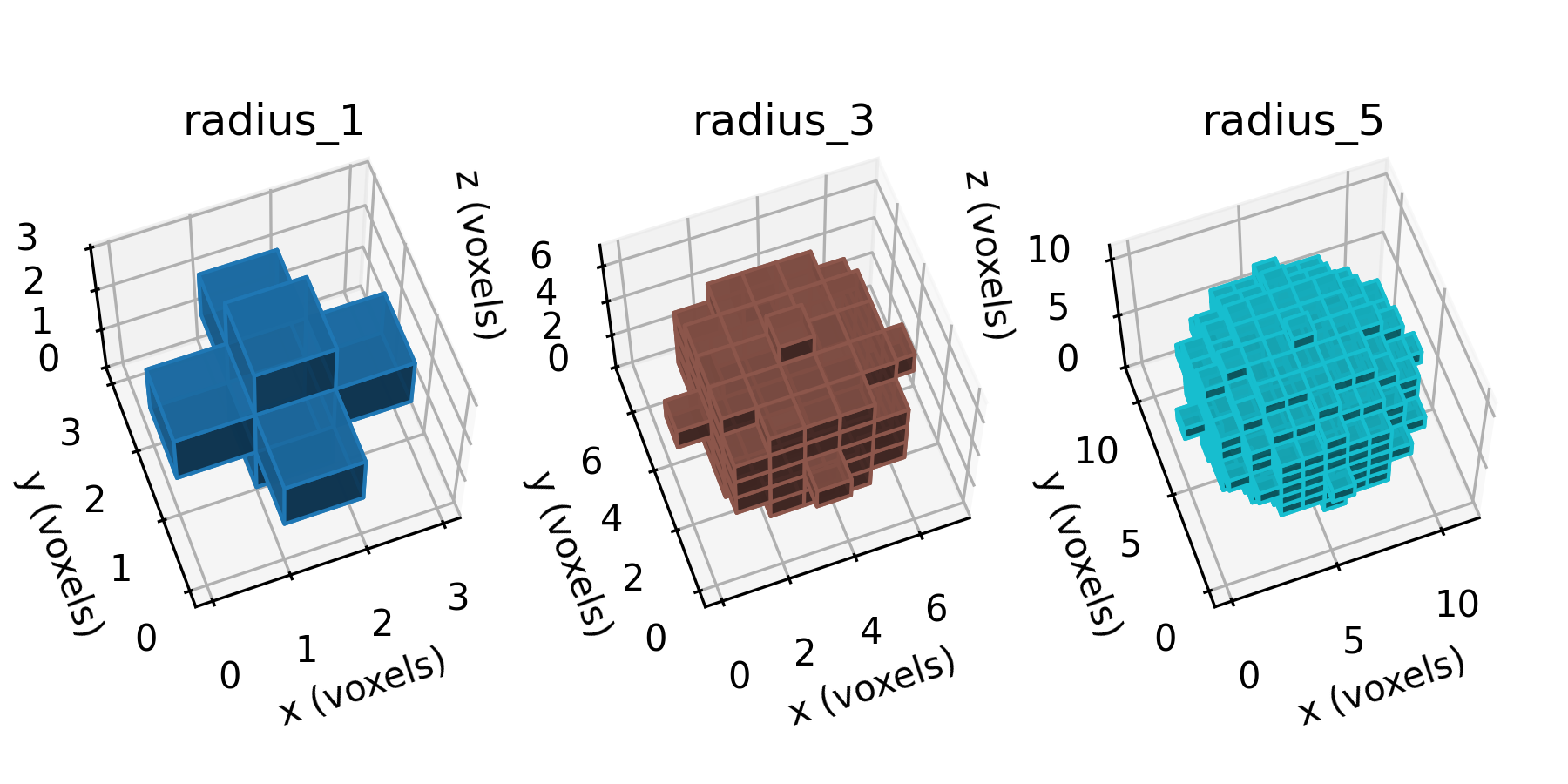
Figure 4.2-1: Sphere segmentations at selected resolutions, shown in the voxel domain.
The radius=1 case has the following data structure,
The radius_1 data structure
spheres["radius_1"]

array([[[0, 0, 0],
        [0, 1, 0],
        [0, 0, 0]],

       [[0, 1, 0],
        [1, 1, 1],
        [0, 1, 0]],

       [[0, 0, 0],
        [0, 1, 0],
        [0, 0, 0]]], dtype=uint8)
Because of large size, the data structures for sphere_3 and
sphere_5 are not shown here.
These segmentations are saved to
automesh
automesh is used to convert the .npy segmentations into .inp meshes.
The radius=1 command and output
automesh mesh hex -i spheres_radius_1.npy -o spheres_radius_1.inp
    automesh 0.5.1
     Reading spheres_radius_1.npy
        Done 23.615µs [2 materials, 27 voxels]
     Meshing voxels into hexahedra
        Done 17.587µs [27 elements, 64 nodes]
     Writing spheres_radius_1.inp
        Done 79.821µs
       Total 495.69µs
The radius=3 command and output
automesh mesh hex -i spheres_radius_3.npy -o spheres_radius_3.inp
    automesh 0.5.1
     Reading spheres_radius_3.npy
        Done 21.733µs [2 materials, 343 voxels]
     Meshing voxels into hexahedra
        Done 42.054µs [343 elements, 512 nodes]
     Writing spheres_radius_3.inp
        Done 160.353µs
       Total 601.691µs
The radius=5 command and output
automesh mesh hex -i spheres_radius_5.npy -o spheres_radius_5.inp
    automesh 0.5.1
     Reading spheres_radius_5.npy
        Done 21.373µs [2 materials, 1331 voxels]
     Meshing voxels into hexahedra
        Done 227.684µs [1331 elements, 1728 nodes]
     Writing spheres_radius_5.inp
        Done 462.64µs
       Total 1.112554ms
Mesh
The spheres_radius_1.inp file
*Heading
 conspire mesh
*Node
1, 0, 0, 0
2, 1, 0, 0
3, 2, 0, 0
4, 3, 0, 0
5, 0, 1, 0
6, 1, 1, 0
7, 2, 1, 0
8, 3, 1, 0
9, 0, 2, 0
10, 1, 2, 0
11, 2, 2, 0
12, 3, 2, 0
13, 0, 3, 0
14, 1, 3, 0
15, 2, 3, 0
16, 3, 3, 0
17, 0, 0, 1
18, 1, 0, 1
19, 2, 0, 1
20, 3, 0, 1
21, 0, 1, 1
22, 1, 1, 1
23, 2, 1, 1
24, 3, 1, 1
25, 0, 2, 1
26, 1, 2, 1
27, 2, 2, 1
28, 3, 2, 1
29, 0, 3, 1
30, 1, 3, 1
31, 2, 3, 1
32, 3, 3, 1
33, 0, 0, 2
34, 1, 0, 2
35, 2, 0, 2
36, 3, 0, 2
37, 0, 1, 2
38, 1, 1, 2
39, 2, 1, 2
40, 3, 1, 2
41, 0, 2, 2
42, 1, 2, 2
43, 2, 2, 2
44, 3, 2, 2
45, 0, 3, 2
46, 1, 3, 2
47, 2, 3, 2
48, 3, 3, 2
49, 0, 0, 3
50, 1, 0, 3
51, 2, 0, 3
52, 3, 0, 3
53, 0, 1, 3
54, 1, 1, 3
55, 2, 1, 3
56, 3, 1, 3
57, 0, 2, 3
58, 1, 2, 3
59, 2, 2, 3
60, 3, 2, 3
61, 0, 3, 3
62, 1, 3, 3
63, 2, 3, 3
64, 3, 3, 3
*Element, type=C3D8, elset=BLOCK1
1, 1, 2, 6, 5, 17, 18, 22, 21
2, 17, 18, 22, 21, 33, 34, 38, 37
3, 33, 34, 38, 37, 49, 50, 54, 53
4, 5, 6, 10, 9, 21, 22, 26, 25
5, 37, 38, 42, 41, 53, 54, 58, 57
6, 9, 10, 14, 13, 25, 26, 30, 29
7, 25, 26, 30, 29, 41, 42, 46, 45
8, 41, 42, 46, 45, 57, 58, 62, 61
9, 2, 3, 7, 6, 18, 19, 23, 22
10, 34, 35, 39, 38, 50, 51, 55, 54
11, 10, 11, 15, 14, 26, 27, 31, 30
12, 42, 43, 47, 46, 58, 59, 63, 62
13, 3, 4, 8, 7, 19, 20, 24, 23
14, 19, 20, 24, 23, 35, 36, 40, 39
15, 35, 36, 40, 39, 51, 52, 56, 55
16, 7, 8, 12, 11, 23, 24, 28, 27
17, 39, 40, 44, 43, 55, 56, 60, 59
18, 11, 12, 16, 15, 27, 28, 32, 31
19, 27, 28, 32, 31, 43, 44, 48, 47
20, 43, 44, 48, 47, 59, 60, 64, 63
*Element, type=C3D8, elset=BLOCK2
21, 21, 22, 26, 25, 37, 38, 42, 41
22, 18, 19, 23, 22, 34, 35, 39, 38
23, 6, 7, 11, 10, 22, 23, 27, 26
24, 22, 23, 27, 26, 38, 39, 43, 42
25, 38, 39, 43, 42, 54, 55, 59, 58
26, 26, 27, 31, 30, 42, 43, 47, 46
27, 23, 24, 28, 27, 39, 40, 44, 43
Because of large size, the mesh structures for sphere_3 and
sphere_5 are not shown here.
Source
spheres.py
spheres.py
r"""This module, spheres.py, creates a voxelized sphere and exports
it as a .npy file.

Example
-------
source ~/autotwin/automesh/.venv/bin/activate
cd book/examples/spheres
python spheres.py
"""

from pathlib import Path
from typing import Final

from matplotlib.colors import LightSource
import matplotlib.pyplot as plt
from mpl_toolkits.mplot3d import Axes3D
import numpy as np


def sphere(radius: int, dtype=np.uint8) -> np.ndarray:
    """Generate a 3D voxelized representation of a sphere.

    Parameters
    ----------
    radius: int
        The radius of the sphere.  Minimum value is 1.

    dtype: data-type, optional
        The data type of the output array.  Default is np.uint8.

    Returns
    -------
    np.ndarray
        A 3D numpy array of shape (2*radius+1, 2*radius+1, 2*radius+1)
        representing the voxelized sphere.  Voxels within the sphere are
        set to 1, and those outside are set to 0.

    Raises
    ------
    ValueError
        If the radius is less than 1.

    Example
    -------
    >>> sphere(radius=1) returns
        array(
            [
                [[0, 0, 0], [0, 1, 0], [0, 0, 0]],
                [[0, 1, 0], [1, 1, 1], [0, 1, 0]],
                [[0, 0, 0], [0, 1, 0], [0, 0, 0]]
            ],
            dtype=uint8
        )

    Reference
    ---------
    Adapted from:
    https://github.com/scikit-image/scikit-image/blob/v0.24.0/skimage/morphology/footprints.py#L763-L833
    """
    if radius < 1:
        raise ValueError("Radius must be >= 1")

    n_voxels_per_side = 2 * radius + 1
    vox_z, vox_y, vox_x = np.mgrid[
        -radius : radius : n_voxels_per_side * 1j,
        -radius : radius : n_voxels_per_side * 1j,
        -radius : radius : n_voxels_per_side * 1j,
    ]
    voxel_radius_squared = vox_x**2 + vox_y**2 + vox_z**2
    result = np.array(voxel_radius_squared <= radius * radius, dtype=dtype)
    return result


# User input begin

spheres = {
    "radius_1": sphere(radius=1),
    "radius_3": sphere(radius=3),
    "radius_5": sphere(radius=5),
}

aa = Path(__file__)
bb = aa.with_suffix(".png")

# Visualize the elements.
width, height = 10, 5
# width, height = 8, 4
# width, height = 6, 3
fig = plt.figure(figsize=(width, height))

el, az, roll = 63, -110, 0
cmap = plt.get_cmap(name="tab10")
# NUM_COLORS = len(spheres)
NUM_COLORS = 10  # consistent with tab10 color scheme
VOXEL_ALPHA: Final[float] = 0.9

colors = cmap(np.linspace(0, 1, NUM_COLORS))
lightsource = LightSource(azdeg=325, altdeg=45)  # azimuth, elevation
# lightsource = LightSource(azdeg=325, altdeg=90)  # azimuth, elevation
DPI: Final[int] = 300  # resolution, dots per inch
SHOW: Final[bool] = False  # turn to True to show the figure on screen
SAVE: Final[bool] = False  # turn to True to save .png and .npy files
# User input end


N_SUBPLOTS = len(spheres)
IDX = 1
for index, (key, value) in enumerate(spheres.items()):
    ax = fig.add_subplot(1, N_SUBPLOTS, index + 1, projection=Axes3D.name)
    ax.voxels(
        value,
        facecolors=colors[index],
        edgecolor=colors[index],
        alpha=VOXEL_ALPHA,
        lightsource=lightsource,
    )
    ax.set_title(key.replace("_", "="))
    IDX += 1

    # Set labels for the axes
    ax.set_xlabel("x (voxels)")
    ax.set_ylabel("y (voxels)")
    ax.set_zlabel("z (voxels)")

    # Set the camera view
    ax.set_aspect("equal")
    ax.view_init(elev=el, azim=az, roll=roll)

    if SAVE:
        cc = aa.with_stem("spheres_" + key)
        dd = cc.with_suffix(".npy")
        # Save the data in .npy format
        np.save(dd, value)
        print(f"Saved: {dd}")

fig.tight_layout()
if SHOW:
    plt.show()

if SAVE:
    fig.savefig(bb, dpi=DPI, bbox_inches="tight")
    print(f"Saved: {bb}")
test_spheres.py
test_spheres.py
r"""This module, test_spheres.py, performs point testing of the sphere module.

Example
-------
source ~/autotwin/automesh/.venv/bin/activate
python -m pytest book/examples/spheres/test_spheres.py
"""

import numpy as np
import pytest

import spheres as sph


def test_sphere():
    """Unit tests for the sphere function."""

    # Assure that radius >=1 assert is raised
    with pytest.raises(ValueError, match="Radius must be >= 1"):
        sph.sphere(radius=0)

    #  Assure radius=1 is correct
    gold_r1 = np.array(
        [
            [[0, 0, 0], [0, 1, 0], [0, 0, 0]],
            [[0, 1, 0], [1, 1, 1], [0, 1, 0]],
            [[0, 0, 0], [0, 1, 0], [0, 0, 0]],
        ],
        dtype=np.uint8,
    )

    result_r1 = sph.sphere(radius=1)
    assert np.all(gold_r1 == result_r1)

    #  Assure radius=2 is correct
    gold_r2 = np.array(
        [
            [
                [0, 0, 0, 0, 0],
                [0, 0, 0, 0, 0],
                [0, 0, 1, 0, 0],
                [0, 0, 0, 0, 0],
                [0, 0, 0, 0, 0],
            ],
            [
                [0, 0, 0, 0, 0],
                [0, 1, 1, 1, 0],
                [0, 1, 1, 1, 0],
                [0, 1, 1, 1, 0],
                [0, 0, 0, 0, 0],
            ],
            [
                [0, 0, 1, 0, 0],
                [0, 1, 1, 1, 0],
                [1, 1, 1, 1, 1],
                [0, 1, 1, 1, 0],
                [0, 0, 1, 0, 0],
            ],
            [
                [0, 0, 0, 0, 0],
                [0, 1, 1, 1, 0],
                [0, 1, 1, 1, 0],
                [0, 1, 1, 1, 0],
                [0, 0, 0, 0, 0],
            ],
            [
                [0, 0, 0, 0, 0],
                [0, 0, 0, 0, 0],
                [0, 0, 1, 0, 0],
                [0, 0, 0, 0, 0],
                [0, 0, 0, 0, 0],
            ],
        ],
        dtype=np.uint8,
    )

    result_r2 = sph.sphere(radius=2)
    assert np.all(gold_r2 == result_r2)

    #  Assure radius=3 is correct
    gold_r3 = np.array(
        [
            [
                [0, 0, 0, 0, 0, 0, 0],
                [0, 0, 0, 0, 0, 0, 0],
                [0, 0, 0, 0, 0, 0, 0],
                [0, 0, 0, 1, 0, 0, 0],
                [0, 0, 0, 0, 0, 0, 0],
                [0, 0, 0, 0, 0, 0, 0],
                [0, 0, 0, 0, 0, 0, 0],
            ],
            [
                [0, 0, 0, 0, 0, 0, 0],
                [0, 0, 1, 1, 1, 0, 0],
                [0, 1, 1, 1, 1, 1, 0],
                [0, 1, 1, 1, 1, 1, 0],
                [0, 1, 1, 1, 1, 1, 0],
                [0, 0, 1, 1, 1, 0, 0],
                [0, 0, 0, 0, 0, 0, 0],
            ],
            [
                [0, 0, 0, 0, 0, 0, 0],
                [0, 1, 1, 1, 1, 1, 0],
                [0, 1, 1, 1, 1, 1, 0],
                [0, 1, 1, 1, 1, 1, 0],
                [0, 1, 1, 1, 1, 1, 0],
                [0, 1, 1, 1, 1, 1, 0],
                [0, 0, 0, 0, 0, 0, 0],
            ],
            [
                [0, 0, 0, 1, 0, 0, 0],
                [0, 1, 1, 1, 1, 1, 0],
                [0, 1, 1, 1, 1, 1, 0],
                [1, 1, 1, 1, 1, 1, 1],
                [0, 1, 1, 1, 1, 1, 0],
                [0, 1, 1, 1, 1, 1, 0],
                [0, 0, 0, 1, 0, 0, 0],
            ],
            [
                [0, 0, 0, 0, 0, 0, 0],
                [0, 1, 1, 1, 1, 1, 0],
                [0, 1, 1, 1, 1, 1, 0],
                [0, 1, 1, 1, 1, 1, 0],
                [0, 1, 1, 1, 1, 1, 0],
                [0, 1, 1, 1, 1, 1, 0],
                [0, 0, 0, 0, 0, 0, 0],
            ],
            [
                [0, 0, 0, 0, 0, 0, 0],
                [0, 0, 1, 1, 1, 0, 0],
                [0, 1, 1, 1, 1, 1, 0],
                [0, 1, 1, 1, 1, 1, 0],
                [0, 1, 1, 1, 1, 1, 0],
                [0, 0, 1, 1, 1, 0, 0],
                [0, 0, 0, 0, 0, 0, 0],
            ],
            [
                [0, 0, 0, 0, 0, 0, 0],
                [0, 0, 0, 0, 0, 0, 0],
                [0, 0, 0, 0, 0, 0, 0],
                [0, 0, 0, 1, 0, 0, 0],
                [0, 0, 0, 0, 0, 0, 0],
                [0, 0, 0, 0, 0, 0, 0],
                [0, 0, 0, 0, 0, 0, 0],
            ],
        ],
        dtype=np.uint8,
    )

    result_r3 = sph.sphere(radius=3)
    assert np.all(gold_r3 == result_r3)
Defeature example: blobs
This worked example applies defeature to a synthetic
segmentation of four circular blobs with random noise, illustrating how the
voxel threshold determines which clusters survive and which are resorbed.
With Python, we created a segmentation of four circular blobs with
noise placed randomly in a bounding box, shown in left of the figure below.
The segmentation file blobs.npy was then used as the input to automesh
with the defeature command. The output file blobs_defeatured.npy is
shown in the right of the figure. The threshold was set to 20 voxels.
The defeature command
automesh defeature -i blobs.npy -o blobs_defeatured.npy -m 20
Both the segmentation files, original and defeatured, were then converted to a mesh and visualized in Hexalab.
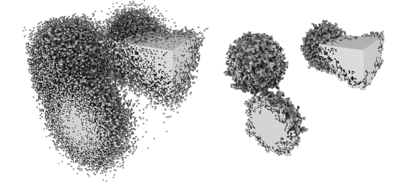
Figure 4.3-1: (left) Four circular blobs with noise (blobs.npy) used as input to
the defeature command, (right) the output defeatured segmentation
(blobs_defeatured.npy).
Source
defeature.py
defeature.py
r"""This module creates spheres and blobs inside of a domain for the purposes
of illustrating the defeature command.

Example:
source ~/autotwin/automesh/.venv/bin/activate
cd ~/autotwin/automesh/book/defeature
python defeature.py
"""

import logging
from pathlib import Path
import random
import subprocess
from typing import Final

import numpy as np

DOMAIN_SIZE: Final[int] = 128
NUM_SPHERES: Final[int] = 4
RADIUS_MAX: Final[int] = 20
FN_SPHERE_STEM = "spheres"
FN_BLOB_STEM = "blobs"

# Configure logging
logging.basicConfig(
    level=logging.INFO,
    format="%(levelname)s: %(message)s",
)


def create_spheres(data: np.ndarray, num_spheres: int, radius_max: int) -> None:
    """Creates random spheres in a 3D binary array.

    Parameters:
        data: A 3D binary array representing the domain.
        num_spheres: The number of spheres to create.
        radius_max: The radius of the spheres.
    """
    shape = data.shape
    (xmin, ymin, zmin) = (0, 0, 0)
    (xmax, ymax, zmax) = (shape[0] - 1, shape[1] - 1, shape[2] - 1)

    for _ in range(num_spheres):
        # Randomly choose a center for the sphere
        center = np.array(
            [
                random.randint(xmin, xmax),
                random.randint(ymin, ymax),
                random.randint(zmin, zmax),
            ]
        )

        # Randomly choose a center for the sphere
        radius = random.randint(1, radius_max)

        # Create a grid of indices
        z, y, x = np.indices(shape)

        # Calculate the distance from the center
        distance = np.sqrt(
            (x - center[0]) ** 2 + (y - center[1]) ** 2 + (z - center[2]) ** 2
        )

        # Set the voxels within the radius to 1
        data[distance <= radius] = 1


def create_blob(data: np.ndarray, center: np.ndarray, radius_max: int) -> None:
    """Creates a sphere-like blob in a 3D binary array.

    Parameters:
        data: A 3D binary array representing the domain.
        center: The center of the blob.
        radius_max: The maximum radius of the blob.
    """

    # Create a grid of indices
    z, y, x = np.indices(data.shape)

    # Calculate the distance from the center
    distance = np.sqrt(
        (x - center[0]) ** 2 + (y - center[1]) ** 2 + (z - center[2]) ** 2
    )

    # Create a random radius for each voxel based on a Gaussian distribution
    radius_variation = np.random.normal(
        loc=radius_max, scale=radius_max * 0.5, size=data.shape
    )

    # Set the voxels to 1 if they are within the radius variation
    data[distance <= radius_variation] = 1


def create_blobs(data: np.ndarray, num_blobs: int, radius_max: int) -> None:
    """Create a number of sphere-like blobs in a 3D binary array.

    Parameters:
    data: A 3D binary array representing the domain.
    num_blobs: The number of blobs to create.
    radius_max: The maximum radius of the blobs.
    """

    shape = data.shape
    (xmin, ymin, zmin) = (0, 0, 0)
    (xmax, ymax, zmax) = (shape[0] - 1, shape[1] - 1, shape[2] - 1)

    for _ in range(num_blobs):
        # Randomly choose a center for the blob
        center = np.array(
            [
                random.randint(xmin, xmax),
                random.randint(ymin, ymax),
                random.randint(zmin, zmax),
            ]
        )

        # Create a blob at the center
        create_blob(data=data, center=center, radius_max=radius_max)


def run_commands(commands: list[list[str]]) -> None:
    """Run a list of commands in the shell, stopping at the first failure.

    Parameters:
        commands: A list of command argument lists to run.

    Raises:
        subprocess.CalledProcessError: If any command exits non-zero. Later
            commands often depend on the output of earlier ones, so
            continuing after a failure would only produce a more confusing
            error downstream.
    """
    for command in commands:
        try:
            logging.info("Running command: %s", " ".join(command))
            result = subprocess.run(command, check=True, capture_output=True, text=True)
            logging.info("Command output: %s", result.stdout)
        except subprocess.CalledProcessError as e:
            logging.error("Error running command:")
            logging.error("Command: %s", " ".join(command))
            logging.error("Return code: %s", e.returncode)
            logging.error("Standard Output: %s", e.stdout)
            logging.error("Standard Error: %s", e.stderr)
            raise


def resolve_automesh() -> Path:
    """Resolve the path to the `automesh` release binary.

    Returns:
        The path to the `automesh` binary.
    """
    automesh = Path("~/autotwin/automesh/target/release/automesh").expanduser()
    assert automesh.is_file(), f"automesh not found at {automesh}"
    return automesh


def mesh_hex_cmd(automesh: Path, input_file: str, output_file: str) -> list[str]:
    """Build an `automesh mesh hex` command with no refinement.

    Parameters:
        automesh: The path to the `automesh` binary.
        input_file: The input segmentation file (`.npy`).
        output_file: The output mesh file (`.exo` or `.mesh`).

    Returns:
        The command as a list of arguments, suitable for `subprocess.run`.
    """
    return [str(automesh), "mesh", "hex", "-i", input_file, "-o", output_file, "-r", "0"]


def spheres():
    """Create and save a 3D binary array with random spheres."""
    # Initialize the domain filled with zeros
    domain = np.zeros((DOMAIN_SIZE, DOMAIN_SIZE, DOMAIN_SIZE), dtype=np.uint8)

    # Create spheres in the domain
    create_spheres(data=domain, num_spheres=NUM_SPHERES, radius_max=RADIUS_MAX)

    # Save the data to a .npy file
    FN_SPHERE = f"{FN_SPHERE_STEM}.npy"

    np.save(FN_SPHERE, domain)
    print(f"The domain with spheres has been saved to:\n{FN_SPHERE}.")

    # Create the mesh with automesh
    automesh = resolve_automesh()

    FN_SPHERE_EXO = f"{FN_SPHERE_STEM}.exo"
    FN_SPHERE_MESH = f"{FN_SPHERE_STEM}.mesh"

    commands = [
        mesh_hex_cmd(automesh, FN_SPHERE, FN_SPHERE_EXO),
        mesh_hex_cmd(automesh, FN_SPHERE, FN_SPHERE_MESH),
    ]

    run_commands(commands=commands)


def blobs():
    """Create and save a 3D binary array with random blobs."""

    # Initialize the domain filled with zeros
    domain = np.zeros((DOMAIN_SIZE, DOMAIN_SIZE, DOMAIN_SIZE), dtype=np.uint8)

    # Create blobs in the domain
    create_blobs(data=domain, num_blobs=NUM_SPHERES, radius_max=RADIUS_MAX)
    # Save the data to a .npy file
    FN_BLOB = f"{FN_BLOB_STEM}.npy"
    FN_BLOB_DEFEATURED = f"{FN_BLOB_STEM}_defeatured.npy"

    np.save(FN_BLOB, domain)
    print(f"The domain with blobs has been saved to:\n{FN_BLOB}.")

    # Create the mesh with automesh
    automesh = resolve_automesh()

    FN_BLOB_EXO = f"{FN_BLOB_STEM}.exo"
    FN_BLOB_MESH = f"{FN_BLOB_STEM}.mesh"
    FN_BLOB_DEFEATURED_EXO = f"{FN_BLOB_STEM}_defeatured.exo"
    FN_BLOB_DEFEATURED_MESH = f"{FN_BLOB_STEM}_defeatured.mesh"

    commands = [
        mesh_hex_cmd(automesh, FN_BLOB, FN_BLOB_EXO),
        mesh_hex_cmd(automesh, FN_BLOB, FN_BLOB_MESH),
        [str(automesh), "defeature", "-i", FN_BLOB, "-o", FN_BLOB_DEFEATURED, "-m", "20"],
        mesh_hex_cmd(automesh, FN_BLOB_DEFEATURED, FN_BLOB_DEFEATURED_EXO),
        mesh_hex_cmd(automesh, FN_BLOB_DEFEATURED, FN_BLOB_DEFEATURED_MESH),
    ]

    run_commands(commands=commands)


if __name__ == "__main__":
    spheres()
    blobs()
Mesh example: Torus
The Stanford bunny and Unit sphere
pages both focus on remesh, which only produces valid output for
triangular surface meshes (see Mesh). Here we look at
the other side of mesh's command chaining: mesh hex smooth, which
generates an all-hexahedral volumetric mesh directly from a segmentation
and smooths it in one command. The shape is a torus — a genus-1, fully
closed solid, distinct from the bunny's open, boundary-having scan and the
sphere's genus-0 shell.
Downloadable Files
Every file on this page is small and reproducible; each is also available for direct download:
| file | description |
|---|---|
| torus.npy | The torus segmentation (see Generating the Torus). |
| torus_raw.inp | The raw (unsmoothed) all-hexahedral mesh (see Chained: mesh hex smooth). |
| torus_smooth.inp | The same mesh after Taubin smoothing, produced by the single chained command below. |
Generating the Torus
The torus is defined implicitly: a voxel at (x, y, z) is filled when
(sqrt(x² + y²) − R)² + z² ≤ r², for major radius R and minor (tube)
radius r. The torus lies flat in the x-y plane, so the segmentation
array needs a much larger extent in x/y (to span the outer diameter)
than in z (to span the tube only).
Voxelizing that implicit inequality directly leaves single-voxel "horns": spurs that touch the torus body only edge- or corner-adjacent, an aliasing artifact of the discretization rather than a feature of the torus itself. Two passes of morphological opening (erosion then dilation, with a 6-connected structuring element) remove them while leaving the ring's connectivity and overall shape unchanged:
torus.py
"""This module, torus.py, creates a voxelized torus segmentation, used to
demonstrate `automesh mesh hex smooth` chaining on a genus-1 shape.

Example
-------
source ~/autotwin/automesh/.venv/bin/activate
cd ~/autotwin/automesh/book/examples/mesh
python torus.py
"""

import numpy as np
from numpy.typing import NDArray

# Torus parameters, in voxel units.
MAJOR_R = 13.0  # distance from the center of the tube to the center of the torus
MINOR_R = 4.0  # radius of the tube
PAD = 2  # voxels of void padding around the torus


def erode(a: NDArray[np.bool_]) -> NDArray[np.bool_]:
    """One step of binary erosion with a 6-connected (face) structuring
    element: a voxel survives only if it and all its face-neighbors are
    filled.  Out-of-bounds neighbors count as empty."""
    out = a.copy()
    for axis in range(3):
        out &= np.roll(a, 1, axis=axis)
        out &= np.roll(a, -1, axis=axis)
        # np.roll wraps around; undo that wraparound by clearing the edge
        # slices it incorrectly pulled in from the opposite side.
        edge_lo = [slice(None)] * 3
        edge_lo[axis] = 0
        out[tuple(edge_lo)] = False
        edge_hi = [slice(None)] * 3
        edge_hi[axis] = -1
        out[tuple(edge_hi)] = False
    return out


def dilate(a: NDArray[np.bool_]) -> NDArray[np.bool_]:
    """One step of binary dilation with a 6-connected (face) structuring
    element: a voxel is filled if it or any face-neighbor is filled."""
    out = a.copy()
    for axis in range(3):
        shifted_up = np.roll(a, 1, axis=axis)
        shifted_down = np.roll(a, -1, axis=axis)
        edge_lo = [slice(None)] * 3
        edge_lo[axis] = 0
        shifted_up[tuple(edge_lo)] = False
        edge_hi = [slice(None)] * 3
        edge_hi[axis] = -1
        shifted_down[tuple(edge_hi)] = False
        out |= shifted_up
        out |= shifted_down
    return out


# The torus lies flat in the x-y plane, so it needs a much larger extent in
# x and y (to span its outer diameter) than in z (to span the tube only).
xy_extent = int(MAJOR_R + MINOR_R) + PAD
z_extent = int(MINOR_R) + PAD
xy_coords = np.arange(-xy_extent, xy_extent + 1)
z_coords = np.arange(-z_extent, z_extent + 1)
x, y, z = np.meshgrid(xy_coords, xy_coords, z_coords, indexing="ij")

rho = np.sqrt(x**2 + y**2) - MAJOR_R
inside = (rho**2 + z**2) <= MINOR_R**2

# Voxelizing a smooth implicit surface leaves single-voxel "horns": spurs
# that touch the torus body only edge- or corner-adjacent, an aliasing
# artifact of the discretization, not a feature of the torus itself.
# Morphological opening (erosion then dilation, twice) removes them while
# leaving the ring's connectivity and overall shape unchanged.
for _ in range(2):
    inside = erode(inside)
for _ in range(2):
    inside = dilate(inside)

segmentation = np.where(inside, 1, 0).astype(np.uint8)

FILE_NAME = "torus.npy"
np.save(FILE_NAME, segmentation)
print(f"Saved {FILE_NAME} with shape {segmentation.shape}.")
Chained: mesh hex smooth
Without chaining, generating and smoothing a hex mesh takes two commands and
an intermediate file. With chaining, it's one command and no intermediate
file — smooth runs immediately on the mesh mesh hex just built, in
memory:
The chained mesh hex smooth command and output
automesh mesh hex -r 0 -i torus.npy -o torus_smooth.inp smooth
    automesh 0.5.1
     Reading torus.npy
       Total 415.949µs
Remark:
-r 0(removing void) must come before-i/-ohere, not after.-raccepts a variable number of IDs, so if it were the last flag before thesmoothsubcommand, it would try to consumesmoothitself as another ID and fail to parse. Placing a single-value flag like-iright after-rcloses off its argument list unambiguously.
For comparison, the unsmoothed mesh:
The unsmoothed mesh hex command and output
automesh mesh hex -r 0 -i torus.npy -o torus_raw.inp
    automesh 0.5.1
     Reading torus.npy
       Total 315.477µs
| raw (3,552 elements) | smoothed (3,552 elements) |
|---|---|
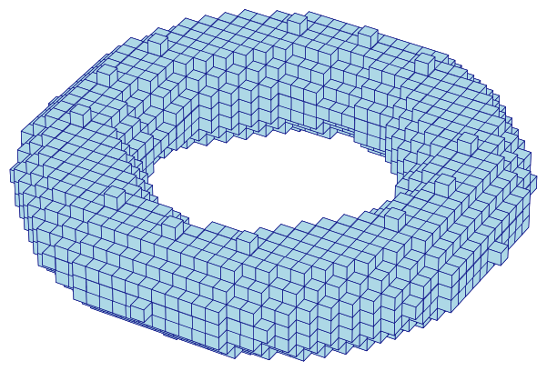 | 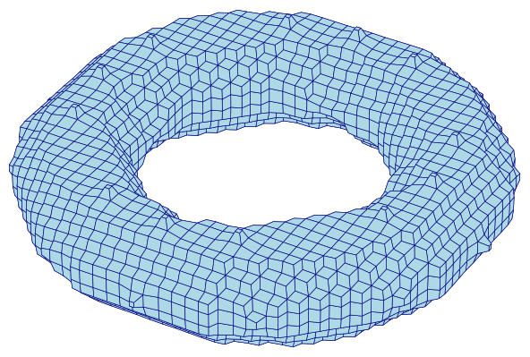 |
Figure 4.4-1: The same 3,552-element hexahedral mesh before (left) and after (right) 20 iterations of Taubin smoothing, chained directly onto meshing. Smoothing does not change the element or node count — it only relocates nodes — so the voxel "staircasing" on the left becomes a smoothed torus on the right.
Smoothing's Effect on Element Quality
Smoothing improves the visual surface, but it is not free: moving nodes off the regular voxel grid distorts elements that were, before smoothing, perfect unit cubes. Metrics quantifies this trade-off:
| metric | raw | smoothed (min) | smoothed (mean) | smoothed (max) |
|---|---|---|---|---|
| minimum scaled Jacobian | 1.000 | 0.500 | 0.933 | 1.000 |
| maximum skew | 0.000 | 0.000 | 0.090 | 0.337 |
| maximum edge ratio | 1.000 | 1.002 | 1.193 | 2.901 |
Every raw element is an identical unit cube, so its metrics are trivially
perfect. After smoothing, most elements stay close to that ideal (mean
scaled Jacobian 0.933), but the worst element — likely near the torus's
tight inner radius, where curvature is highest — drops to 0.500. For this
example that's still a well-shaped element, but it illustrates why
automesh smooth's output is worth checking with metrics before it's
used, not just visually inspected.
Chaining remesh After mesh hex smooth Fails
mesh hex smooth also accepts a further remesh subcommand at the command
line, but running it always fails on this torus, exactly as documented in
Mesh — remesh requires triangular
connectivity, and a hex mesh has none:
The mesh hex smooth remesh command
automesh mesh hex -r 0 -i torus.npy -o torus_bad.inp smooth remesh
The error message
Error: connectivity contains a non-triangular block.
Remeshing after smoothing is only meaningful for mesh tri (a triangular
isosurface, not a hex volume) — see the Stanford bunny
and Unit sphere pages for that case worked in full.
Source
The figures on this page are produced by the following script, which reads
the segmentation directly (for the raw voxel view) and the smoothed .inp
mesh (extracting its exterior quad faces for the smoothed view):
torus_figures.py
r"""This module, torus_figures.py, renders the torus segmentation and the
resulting hexahedral meshes (raw and Taubin-smoothed) used in the torus mesh
hex smooth example.

Example
-------
source ~/autotwin/automesh/.venv/bin/activate
cd ~/autotwin/automesh/book/examples/mesh
python torus.py
automesh mesh hex -r 0 -i torus.npy -o torus_raw.inp
automesh mesh hex -r 0 -i torus.npy -o torus_smooth.inp smooth
python torus_figures.py

Output
------
The `torus_raw.png` and `torus_smooth.png` visualization files, written next
to this script.
"""

from collections import Counter
from pathlib import Path
from typing import Final

import matplotlib.pyplot as plt
from mpl_toolkits.mplot3d.art3d import Poly3DCollection
import numpy as np
from numpy.typing import NDArray
from PIL import Image

# Shared "hero" view so only the mesh changes between figures.
ELEV: Final[float] = 35.0
AZIM: Final[float] = -60.0
FACECOLOR: Final[str] = "lightblue"
EDGECOLOR: Final[str] = "navy"

# Local (0-indexed) face node order for an Abaqus C3D8 hexahedron.
C3D8_FACES: Final[tuple[tuple[int, int, int, int], ...]] = (
    (0, 1, 2, 3),
    (4, 5, 6, 7),
    (0, 1, 5, 4),
    (1, 2, 6, 5),
    (2, 3, 7, 6),
    (3, 0, 4, 7),
)


def read_inp_hex(
    path: Path,
) -> tuple[dict[int, tuple[float, float, float]], list[tuple[int, ...]]]:
    """Reads nodes and C3D8 element connectivity from an Abaqus .inp file."""
    nodes: dict[int, tuple[float, float, float]] = {}
    elements: list[tuple[int, ...]] = []
    section = None
    for line in path.read_text().splitlines():
        stripped = line.strip()
        if not stripped:
            continue
        if stripped.startswith("*"):
            lower = stripped.lower()
            section = (
                "node"
                if lower.startswith("*node")
                else "element"
                if lower.startswith("*element")
                else None
            )
            continue
        parts = [p.strip() for p in stripped.split(",")]
        if section == "node":
            nodes[int(parts[0])] = tuple(float(v) for v in parts[1:4])
        elif section == "element":
            ids = [int(p) for p in parts]
            elements.append(tuple(ids[1:9]))
    return nodes, elements


def exterior_quads(
    nodes: dict[int, tuple[float, float, float]],
    elements: list[tuple[int, ...]],
) -> list[NDArray[np.float64]]:
    """Returns the mesh's exterior quad faces, each as a (4, 3) coordinate
    array.  A face is exterior if it belongs to exactly one hex element."""
    face_count: Counter[frozenset[int]] = Counter()
    for elem in elements:
        for face in C3D8_FACES:
            face_count[frozenset(elem[i] for i in face)] += 1

    quads = []
    seen: set[frozenset[int]] = set()
    for elem in elements:
        for face in C3D8_FACES:
            node_ids = tuple(elem[i] for i in face)
            key = frozenset(node_ids)
            if face_count[key] == 1 and key not in seen:
                seen.add(key)
                quads.append(np.array([nodes[n] for n in node_ids]))
    return quads


def crop_to_content(path: Path, margin: int = 10) -> None:
    """Crops a saved PNG to its non-white content, since matplotlib's
    `bbox_inches="tight"` does not shrink the whitespace 3D axes leave
    around a plot even with the axes turned off."""
    image = Image.open(path).convert("RGB")
    array = np.asarray(image)
    non_white = np.any(array != 255, axis=-1)
    rows = np.where(non_white.any(axis=1))[0]
    cols = np.where(non_white.any(axis=0))[0]
    top = max(rows.min() - margin, 0)
    bottom = min(rows.max() + margin + 1, array.shape[0])
    left = max(cols.min() - margin, 0)
    right = min(cols.max() + margin + 1, array.shape[1])
    image.crop((left, top, right, bottom)).save(path)


def render_quads(
    quads: list[NDArray[np.float64]],
    bounds: tuple[NDArray[np.float64], NDArray[np.float64]],
    out_path: Path,
) -> None:
    """Renders a list of quad faces as a shaded 3D surface, framed to the
    given (mins, maxs) bounds rather than the quads' own extent, so this
    plot shares an identical scale with a companion `render_voxels` plot."""
    mins, maxs = bounds
    fig = plt.figure(figsize=(6, 6))
    ax = fig.add_subplot(projection="3d")
    collection = Poly3DCollection(
        quads, facecolor=FACECOLOR, edgecolor=EDGECOLOR, linewidths=0.3
    )
    ax.add_collection3d(collection)
    ax.set_xlim(mins[0], maxs[0])
    ax.set_ylim(mins[1], maxs[1])
    ax.set_zlim(mins[2], maxs[2])
    ax.set_box_aspect(tuple(maxs - mins))
    ax.view_init(elev=ELEV, azim=AZIM)
    ax.set_axis_off()
    fig.subplots_adjust(left=0, right=1, bottom=0, top=1)
    fig.savefig(out_path, dpi=150, bbox_inches="tight", pad_inches=0.02)
    plt.close(fig)
    crop_to_content(out_path)
    print(f"wrote {out_path} ({len(quads)} quads)")


def render_voxels(
    filled: NDArray[np.bool_],
    bounds: tuple[NDArray[np.float64], NDArray[np.float64]],
    out_path: Path,
) -> None:
    """Renders a segmentation's occupied voxels directly, as raw cubes,
    framed to the given (mins, maxs) bounds."""
    mins, maxs = bounds
    fig = plt.figure(figsize=(6, 6))
    ax = fig.add_subplot(projection="3d")
    ax.voxels(filled, facecolor=FACECOLOR, edgecolor=EDGECOLOR, linewidth=0.3)
    ax.set_xlim(mins[0], maxs[0])
    ax.set_ylim(mins[1], maxs[1])
    ax.set_zlim(mins[2], maxs[2])
    ax.set_box_aspect(tuple(maxs - mins))
    ax.view_init(elev=ELEV, azim=AZIM)
    ax.set_axis_off()
    fig.subplots_adjust(left=0, right=1, bottom=0, top=1)
    fig.savefig(out_path, dpi=150, bbox_inches="tight", pad_inches=0.02)
    plt.close(fig)
    crop_to_content(out_path)
    print(f"wrote {out_path}")


if __name__ == "__main__":
    filled = np.load(Path("torus.npy")) != 0
    # Both figures share this one reference bounding box (the raw voxel
    # grid's own extent), so they render at an identical scale: same
    # box_aspect, same axis limits, same figure size and DPI.
    bounds = (np.zeros(3), np.array(filled.shape, dtype=float))

    render_voxels(filled, bounds, Path("torus_raw.png"))

    smooth_nodes, smooth_elements = read_inp_hex(Path("torus_smooth.inp"))
    quads = exterior_quads(smooth_nodes, smooth_elements)
    render_quads(quads, bounds, Path("torus_smooth.png"))
Remesh example: unit sphere
This worked example applies remesh to an analytic unit sphere
(radius ≈ 1). Because a sphere has nearly constant curvature, uniform and
adaptive sizing produce almost the same result here — a useful baseline before
the Stanford bunny, where they differ.
The input mesh
Download the example mesh: sphere_radius_1.stl
(binary format, 54 kB)
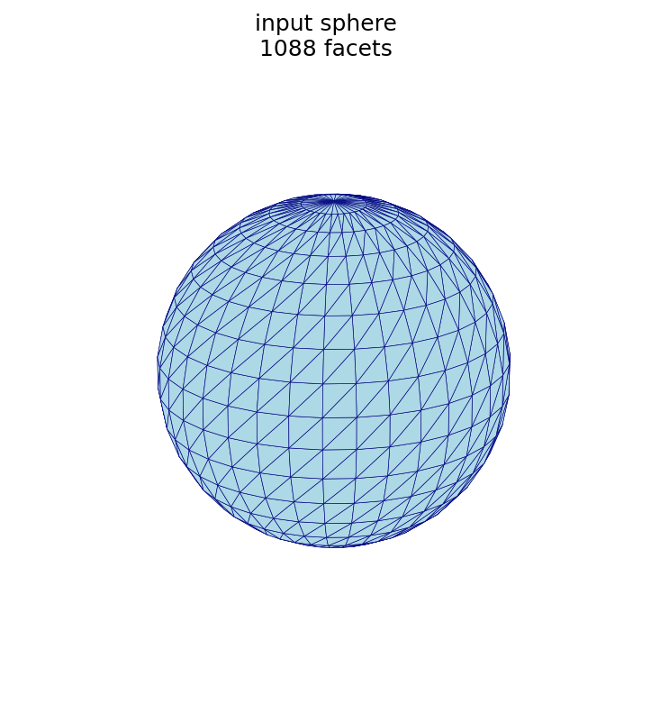
Statistics
| quantity | symbol | value |
|---|---|---|
| facets (triangles) | 1,088 | |
| points (vertices) | 546 | |
| edges | 1,632 |
The mean triangle edge length is 0.178, and most edges cluster near it (see the edge-length histogram in the next section).
Relationship to triangular subdivision
The Subdivision section gives the recursive relationships for one refinement of a closed triangular mesh:
These relationships preserve two invariants of any closed triangular surface, both of which the example sphere satisfies:
- Edge–face relationship, : every triangle has three edges and every edge is shared by two triangles, so . ✓
- Euler characteristic, for a genus-0 (sphere-like) surface: . ✓
These statistics, and the histograms below, are produced by the figure script at the end of this page.
Default remesh
Running remesh with no mode or size uses uniform sizing at the mean edge
length of the input, which regularizes the surface at its existing resolution:
the triangles become more uniform in size and shape while the facet count stays
close to the input.
The default remesh command
automesh remesh -i sphere_radius_1.stl -o sphere_default.stl
| base (1,088 facets) | default (948 facets) |
|---|---|
| 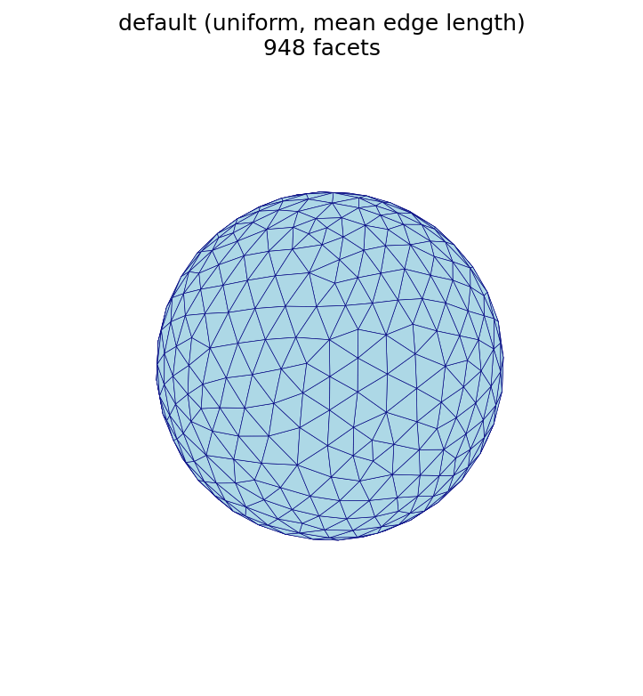 |
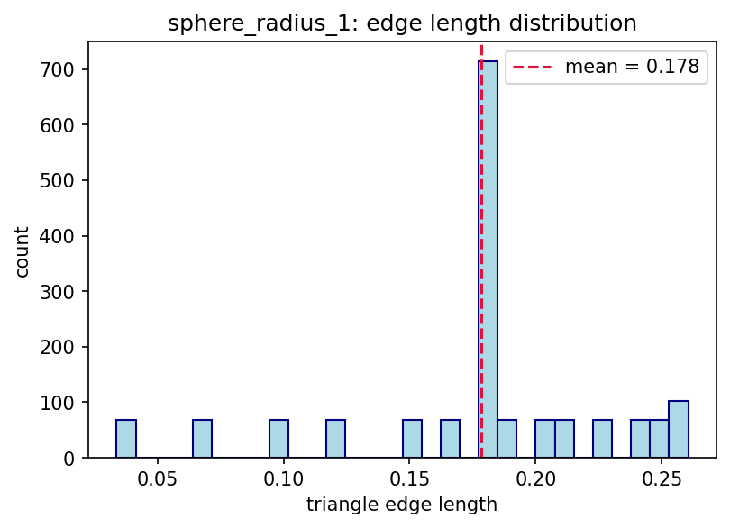 | 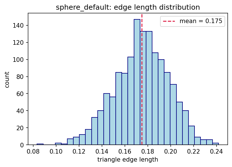 |
The histograms show the effect of remeshing on triangle edge lengths: the base mesh has an irregular, spiky distribution, while the default remesh produces a tighter, bell-shaped distribution centered near the mean edge length.
Uniform sizing: coarse vs. fine
A larger target edge length produces fewer, larger triangles; a smaller target edge length produces many more, smaller triangles.
The coarse and fine remesh commands
automesh remesh -i sphere_radius_1.stl -o sphere_uniform_coarse.stl uniform -s 0.35
automesh remesh -i sphere_radius_1.stl -o sphere_uniform_fine.stl   uniform -s 0.08
| base (1,088 facets) | coarse, -s 0.35 (440 facets) | fine, -s 0.08 (4,744 facets) |
|---|---|---|
| 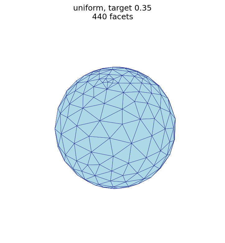 | 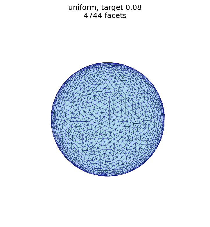 |
Effect of the number of iterations
More iterations make the triangles more uniform, but with strongly diminishing
returns. The sphere is remeshed at the default target edge length for a range of
--iterations values, one output per value:
The six remesh commands, one per iteration count
automesh remesh -i sphere_radius_1.stl -o sphere_n1.stl   uniform -n 1
automesh remesh -i sphere_radius_1.stl -o sphere_n5.stl   uniform -n 5
automesh remesh -i sphere_radius_1.stl -o sphere_n10.stl  uniform -n 10
automesh remesh -i sphere_radius_1.stl -o sphere_n20.stl  uniform -n 20
automesh remesh -i sphere_radius_1.stl -o sphere_n50.stl  uniform -n 50
automesh remesh -i sphere_radius_1.stl -o sphere_n100.stl uniform -n 100
Measuring the edge-length coefficient of variation of each result (CoV , smaller is more uniform) gives:
iterations -n | facets | mean edge | CoV |
|---|---|---|---|
| 1 | 1,380 | 0.154 | 26.6% |
| 5 (default) | 948 | 0.175 | 13.4% |
| 10 | 856 | 0.183 | 9.8% |
| 20 | 846 | 0.184 | 9.7% |
| 50 | 838 | 0.185 | 9.6% |
| 100 | 830 | 0.186 | 9.6% |
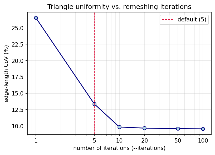
Most of the improvement happens within the first ~10 passes; beyond that the CoV
plateaus at an irreducible floor (≈ 9.6% here — a sphere cannot be tiled with
perfectly equal edges), so additional iterations cost time without making the
triangles measurably more uniform. For this mesh, -n 10 to -n 20 is a
practical sweet spot.
The same trend is visible in the meshes themselves — the triangulation grows more regular from 1 to 10 iterations:
-n 1 (1,380 facets) | -n 5 (948 facets) | -n 10 (856 facets) |
|---|---|---|
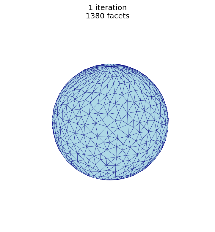 | 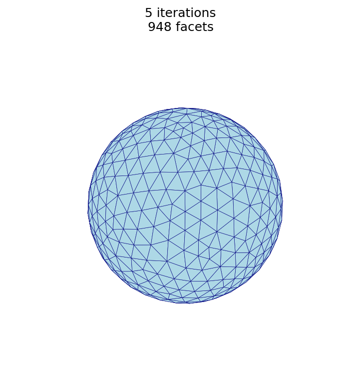 | 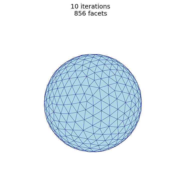 |
This study is produced by the
remesh_iterations.py script shown at the end of the
page.
Uniform vs. adaptive
The uniform and adaptive remesh commands
automesh remesh -i sphere_radius_1.stl -o sphere_uniform.stl  uniform  -s 0.18
automesh remesh -i sphere_radius_1.stl -o sphere_adaptive.stl adaptive --minimum 0.05 --maximum 0.30
uniform, -s 0.18 (910 facets) | adaptive, 0.05–0.30 (458 facets) |
|---|---|
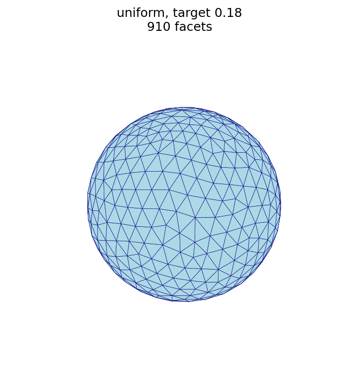 | 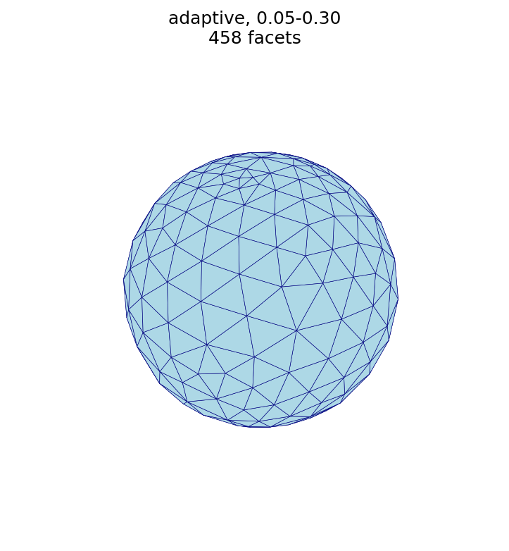 |
Note. A sphere has (nearly) constant curvature, so curvature-adaptive sizing produces an almost uniform result here — the two meshes above look similar. On a model with varying curvature (sharp features together with flat regions), adaptive sizing refines the high-curvature regions and coarsens the flat ones, which uniform sizing cannot do. See the Stanford bunny example for a mesh where uniform and adaptive sizing differ visibly.
Figure script
The figures on this page are produced by the following script, which reads each STL surface and renders it with a matched camera.
remesh_figures.py
r"""This module, remesh_figures.py, renders the surface triangulations used in
the Remesh section of the documentation.  It reads the input sphere and each
remeshed output (produced by `automesh remesh`) and saves a matched-camera PNG
of every mesh, so the effect of uniform and adaptive sizing can be compared
side by side.

Example
-------
source ~/autotwin/automesh/.venv/bin/activate
cd ~/autotwin/automesh/book/examples/remesh
# regenerate the remeshed STL files (binary STL) if needed:
#   automesh remesh -i sphere_radius_1.stl -o sphere_uniform_coarse.stl uniform -s 0.35
#   automesh remesh -i sphere_radius_1.stl -o sphere_uniform_fine.stl   uniform -s 0.08
#   automesh remesh -i sphere_radius_1.stl -o sphere_uniform.stl        uniform -s 0.18
#   automesh remesh -i sphere_radius_1.stl -o sphere_adaptive.stl       adaptive --minimum 0.05 --maximum 0.30
python remesh_figures.py

Output
------
The `*.png` visualization files, one per mesh, written next to this script.
"""

# standard library
import struct
from pathlib import Path
from typing import Final

# third-party library
import matplotlib.pyplot as plt
from mpl_toolkits.mplot3d.art3d import Poly3DCollection
import numpy as np
from numpy.typing import NDArray

# Shared view so triangle-size differences (not camera changes) are what the
# reader sees between figures.
ELEV: Final[float] = 20.0
AZIM: Final[float] = -60.0
LIMIT: Final[float] = 1.05  # sphere radius ~1, small margin
FACECOLOR: Final[str] = "lightblue"
EDGECOLOR: Final[str] = "navy"


def read_stl(path: Path) -> NDArray[np.float64]:
    """Reads triangular facets from an STL file, returning an array of shape
    (n_facets, 3, 3).  Binary and ASCII STL are both supported; the format is
    detected by sniffing the leading bytes."""
    data = path.read_bytes()
    is_ascii = data[:6].lower().startswith(b"solid") and b"facet" in data[:512]
    if is_ascii:
        return _read_ascii(data.decode("ascii", errors="replace"))
    return _read_binary(data)


def _read_binary(data: bytes) -> NDArray[np.float64]:
    """Reads a binary STL (80-byte header, uint32 count, 50 bytes per facet)."""
    (n_facets,) = struct.unpack_from("<I", data, 80)
    facets = np.empty((n_facets, 3, 3), dtype=np.float64)
    offset = 84
    for i in range(n_facets):
        # 12 floats: normal (3) + three vertices (9); trailing uint16 attribute.
        values = struct.unpack_from("<12f", data, offset)
        facets[i] = np.array(values[3:12]).reshape(3, 3)
        offset += 50
    return facets


def _read_ascii(text: str) -> NDArray[np.float64]:
    """Reads an ASCII STL, collecting every `vertex` triple into facets."""
    verts = []
    for line in text.splitlines():
        tokens = line.split()
        if tokens and tokens[0] == "vertex":
            verts.append([float(v) for v in tokens[1:4]])
    return np.array(verts, dtype=np.float64).reshape(-1, 3, 3)


def topology(facets: NDArray[np.float64]) -> tuple[int, int, int]:
    """Returns (faces, edges, vertices) for a triangular surface mesh, where
    coincident vertices are merged and each undirected edge is counted once."""
    faces = len(facets)
    keyed = np.round(facets.reshape(-1, 3), 6)
    _, inverse = np.unique(keyed, axis=0, return_inverse=True)
    ids = inverse.reshape(faces, 3)
    edges = set()
    for a, b, c in ids:
        for u, v in ((a, b), (b, c), (c, a)):
            edges.add((int(min(u, v)), int(max(u, v))))
    vertices = int(ids.max()) + 1
    return faces, len(edges), vertices


def edge_lengths(facets: NDArray[np.float64]) -> NDArray[np.float64]:
    """Returns the length of every unique undirected edge in the mesh."""
    keyed = np.round(facets.reshape(-1, 3), 6)
    coords, inverse = np.unique(keyed, axis=0, return_inverse=True)
    ids = inverse.reshape(len(facets), 3)
    seen = set()
    lengths = []
    for tri, (a, b, c) in zip(facets, ids):
        for (u, v), (p, q) in (((a, b), (0, 1)), ((b, c), (1, 2)), ((c, a), (2, 0))):
            key = (int(min(u, v)), int(max(u, v)))
            if key not in seen:
                seen.add(key)
                lengths.append(float(np.linalg.norm(tri[p] - tri[q])))
    return np.array(lengths)


def render_histogram(stl: Path, out_name: str) -> None:
    """Saves a histogram of the triangle edge lengths of the given mesh."""
    lengths = edge_lengths(read_stl(stl))
    fig, ax = plt.subplots(figsize=(6, 4))
    ax.hist(lengths, bins=30, color=FACECOLOR, edgecolor=EDGECOLOR)
    ax.axvline(
        lengths.mean(),
        color="crimson",
        linestyle="--",
        linewidth=1.5,
        label=f"mean = {lengths.mean():.3f}",
    )
    ax.set_xlabel("triangle edge length")
    ax.set_ylabel("count")
    ax.set_title(f"{stl.stem}: edge length distribution")
    ax.legend()
    png = stl.with_name(out_name)
    fig.savefig(png, dpi=150, bbox_inches="tight")
    plt.close(fig)
    print(f"wrote {png.name} ({len(lengths)} edges)")


def render(stl: Path, title: str) -> None:
    """Renders a single STL surface triangulation to a PNG next to it."""
    facets = read_stl(stl)
    fig = plt.figure(figsize=(6, 6))
    ax = fig.add_subplot(111, projection="3d")
    surface = Poly3DCollection(
        facets, facecolor=FACECOLOR, edgecolor=EDGECOLOR, linewidths=0.3, alpha=1.0
    )
    ax.add_collection3d(surface)
    ax.set_xlim(-LIMIT, LIMIT)
    ax.set_ylim(-LIMIT, LIMIT)
    ax.set_zlim(-LIMIT, LIMIT)
    ax.set_box_aspect((1, 1, 1))
    ax.view_init(elev=ELEV, azim=AZIM)
    ax.set_axis_off()
    ax.set_title(f"{title}\n{len(facets)} facets", fontsize=12)
    png = stl.with_suffix(".png")
    fig.savefig(png, dpi=150, bbox_inches="tight")
    plt.close(fig)
    print(f"wrote {png.name} ({len(facets)} facets)")


def main() -> None:
    here = Path(__file__).resolve().parent
    figures = {
        "sphere_radius_1": "input sphere",
        "sphere_n1": "1 iteration",
        "sphere_n5": "5 iterations",
        "sphere_n10": "10 iterations",
        "sphere_default": "default (uniform, mean edge length)",
        "sphere_uniform_coarse": "uniform, target 0.35",
        "sphere_uniform_fine": "uniform, target 0.08",
        "sphere_uniform": "uniform, target 0.18",
        "sphere_adaptive": "adaptive, 0.05-0.30",
    }
    for stem, title in figures.items():
        stl = here / f"{stem}.stl"
        if stl.exists():
            render(stl, title)
        else:
            print(f"skipping {stl.name} (not found)")

    # Edge-length histograms and topology summary for the base and default meshes.
    histograms = {
        "sphere_radius_1": "sphere_edge_histogram.png",
        "sphere_default": "sphere_default_histogram.png",
    }
    for stem, out_name in histograms.items():
        stl = here / f"{stem}.stl"
        if stl.exists():
            render_histogram(stl, out_name)
            faces, edges, vertices = topology(read_stl(stl))
            print(
                f"{stl.name}: F={faces} E={edges} V={vertices} "
                f"(V - E + F = {vertices - edges + faces})"
            )


if __name__ == "__main__":
    main()
Iteration study script
The effect-of-iterations table and plot
are produced by the following script, which remeshes the sphere at several
--iterations values and measures the edge-length coefficient of variation:
remesh_iterations.py
r"""This module, remesh_iterations.py, studies how the number of remeshing
iterations affects triangle uniformity.  It remeshes the example sphere at the
default target edge length (mean edge length) for a range of `--iterations`
values, measures the edge-length coefficient of variation (CoV = std / mean) of
each result, and plots CoV versus the number of iterations.

Example
-------
source ~/autotwin/automesh/.venv/bin/activate
cd ~/autotwin/automesh/book/examples/remesh
# `automesh` must be on the PATH (e.g. target/release)
python remesh_iterations.py

Output
------
The `sphere_iterations.png` plot, written next to this script, and a summary
table printed to the terminal.
"""

import os
import shutil
import struct
import subprocess
import tempfile
from pathlib import Path

import matplotlib.pyplot as plt
import numpy as np
from numpy.typing import NDArray

ITERATIONS = [1, 5, 10, 20, 50, 100]
FACECOLOR = "lightblue"
EDGECOLOR = "navy"


def automesh_binary() -> str:
    """Locates the `automesh` executable: the AUTOMESH environment variable, then
    the PATH, then the repository's target/release build."""
    candidate = os.environ.get("AUTOMESH") or shutil.which("automesh")
    if candidate:
        return candidate
    fallback = Path(__file__).resolve().parents[2] / "target" / "release" / "automesh"
    if fallback.exists():
        return str(fallback)
    raise FileNotFoundError(
        "could not find `automesh`; set AUTOMESH or add it to the PATH"
    )


def read_stl(path: Path) -> NDArray[np.float64]:
    """Reads triangular facets from a binary STL file."""
    data = path.read_bytes()
    (n_facets,) = struct.unpack_from("<I", data, 80)
    facets = np.empty((n_facets, 3, 3), dtype=np.float64)
    offset = 84
    for i in range(n_facets):
        values = struct.unpack_from("<12f", data, offset)
        facets[i] = np.array(values[3:12]).reshape(3, 3)
        offset += 50
    return facets


def edge_lengths(facets: NDArray[np.float64]) -> NDArray[np.float64]:
    """Returns the length of every unique undirected edge in the mesh."""
    keyed = np.round(facets.reshape(-1, 3), 6)
    _, inverse = np.unique(keyed, axis=0, return_inverse=True)
    ids = inverse.reshape(len(facets), 3)
    seen = set()
    lengths = []
    for tri, (a, b, c) in zip(facets, ids):
        for (u, v), (p, q) in (((a, b), (0, 1)), ((b, c), (1, 2)), ((c, a), (2, 0))):
            key = (int(min(u, v)), int(max(u, v)))
            if key not in seen:
                seen.add(key)
                lengths.append(float(np.linalg.norm(tri[p] - tri[q])))
    return np.array(lengths)


def main() -> None:
    here = Path(__file__).resolve().parent
    source = here / "sphere_radius_1.stl"
    automesh = automesh_binary()
    covs, facet_counts = [], []
    print(f"{'n':>4} {'facets':>7} {'mean':>7} {'CoV%':>6}")
    with tempfile.TemporaryDirectory() as tmp:
        for n in ITERATIONS:
            out = Path(tmp) / f"n{n}.stl"
            subprocess.run(
                [automesh, "remesh", "-i", str(source), "-o", str(out),
                 "uniform", "-n", str(n)],
                check=True, capture_output=True,
            )
            facets = read_stl(out)
            lengths = edge_lengths(facets)
            cov = 100.0 * lengths.std() / lengths.mean()
            covs.append(cov)
            facet_counts.append(len(facets))
            print(f"{n:>4} {len(facets):>7} {lengths.mean():>7.4f} {cov:>6.1f}")

    fig, ax = plt.subplots(figsize=(6, 4))
    ax.plot(ITERATIONS, covs, "o-", color=EDGECOLOR, markerfacecolor=FACECOLOR)
    ax.set_xscale("log")
    ax.set_xticks(ITERATIONS)
    ax.get_xaxis().set_major_formatter(plt.ScalarFormatter())
    ax.set_xlabel("number of iterations (--iterations)")
    ax.set_ylabel("edge-length CoV (%)")
    ax.set_title("Triangle uniformity vs. remeshing iterations")
    ax.axvline(5, color="crimson", linestyle="--", linewidth=1.0, label="default (5)")
    ax.legend()
    ax.grid(True, which="both", alpha=0.3)
    png = here / "sphere_iterations.png"
    fig.savefig(png, dpi=150, bbox_inches="tight")
    plt.close(fig)
    print(f"wrote {png.name}")


if __name__ == "__main__":
    main()
Remesh example: Stanford bunny
The Unit sphere page uses an analytic sphere, whose constant
curvature makes uniform and adaptive sizing behave almost identically. Here, we
work a second, more realistic example: the Stanford bunny, a scanned surface
with sharply varying curvature (ears, folds, paws) and, like most raw scans, a
few holes. It shows how every remesh parameter behaves on a real mesh.
The Stanford bunny is a classic computer-graphics test model, originally scanned by Greg Turk and Marc Levoy at Stanford University in 1994.
Download
The mesh used here is the cleaned bunny from Alec Jacobson's community
common-3d-test-models repository, mirrored on OneDrive for convenience.
Each checksum below shows the first 12 hex characters of the sha256.
stanford-bunny.obj(OBJ, 69,451 triangles, sha2561eb35d1e21ce...) — hosted atOneDrive/automesh/data/stanford-bunny.obj- backup: Alec Jacobson's repository
remesh reads STL (ASCII or binary), not OBJ, so convert the downloaded file
once with the obj_to_binary_stl.py helper (shown
at the end of this page), producing stanford_bunny.stl. All commands on this
page use that converted file.
The OBJ to STL conversion command
python obj_to_binary_stl.py stanford-bunny.obj stanford_bunny.stl
Alternatively, skip the conversion step and download the same file pre-converted:
stanford_bunny.stl(binary STL, pre-converted, sha256909348a1c93e...) — hosted atOneDrive/automesh/data/stanford_bunny.stl
This is the exact output of the command above; either path produces the same
stanford_bunny.stl used throughout the rest of this page.
The input mesh
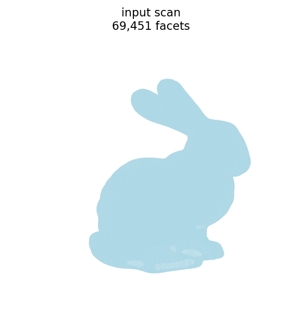
| quantity | symbol | value |
|---|---|---|
| facets (triangles) | 69,451 | |
| points (vertices) | 34,834 | |
| edges | 104,288 | |
| boundary loops (holes) | 5 |
The triangle edge lengths of the scan cluster near a mean of ≈ 0.0015:
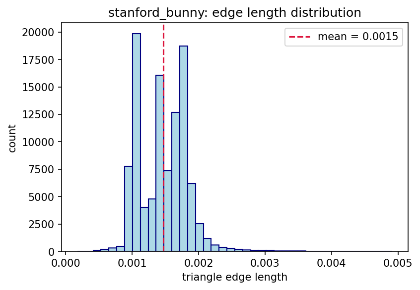
Unlike the sphere, the bunny is not watertight. It is a single connected, manifold, genus-0 surface, but it is open: the base has five boundary loops (holes) left by the scanner. Consequently the closed-surface identities from the sphere example do not hold here:
- is odd, whereas a closed triangular mesh requires and therefore an even facet count.
- The Euler characteristic is (equivalently with genus and holes), rather than the of a closed sphere.
Remeshing handles the open surface without trouble; the boundary loops are preserved through remeshing.
Uniform sizing (--size)
The target edge length sets the triangle size. A smaller --size produces more,
smaller triangles; a larger --size produces fewer, larger triangles.
The uniform remesh commands
automesh remesh -i stanford_bunny.stl -o bunny_uniform_fine.stl   uniform -s 0.004 -n 20
automesh remesh -i stanford_bunny.stl -o bunny_uniform_coarse.stl uniform -s 0.006 -n 20
fine, -s 0.004 (7,715 facets) | coarse, -s 0.006 (3,528 facets) |
|---|---|
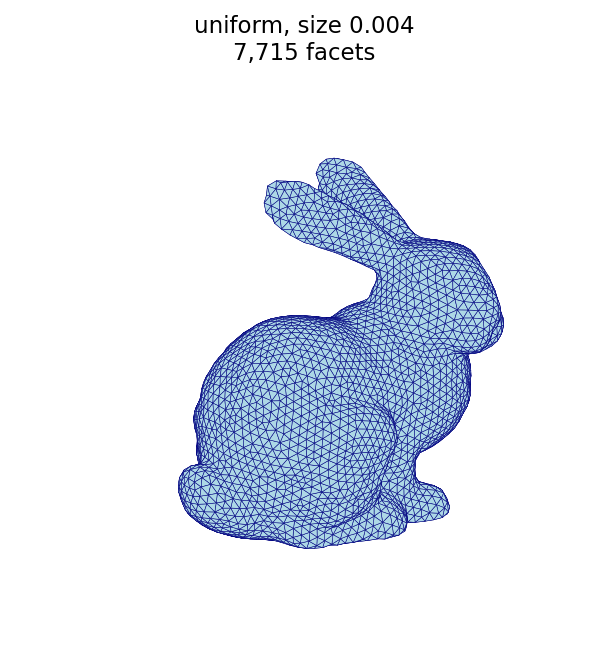 | 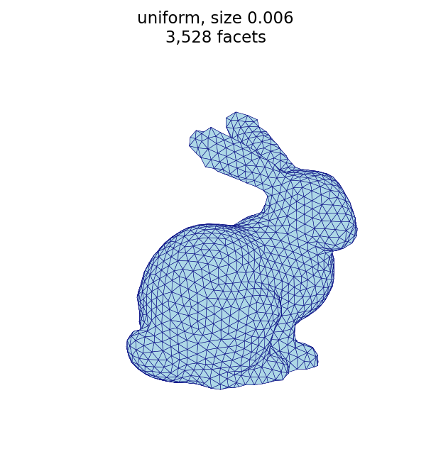 |
Iterations and coarsening (--iterations)
The bunny highlights an effect the sphere did not: coarsening a fine mesh to a
large target edge length is iteration-limited. Each pass can only collapse
edges so much, so reaching a coarse target from a dense input takes several
passes. At the same target -s 0.006, five iterations barely coarsen the
69,451-triangle input, while twenty iterations reach the target:
The iteration remesh commands
automesh remesh -i stanford_bunny.stl -o bunny_iter_n5.stl        uniform -s 0.006 -n 5
automesh remesh -i stanford_bunny.stl -o bunny_uniform_coarse.stl uniform -s 0.006 -n 20
-n 5 (29,826 facets) | -n 20 (3,528 facets) |
|---|---|
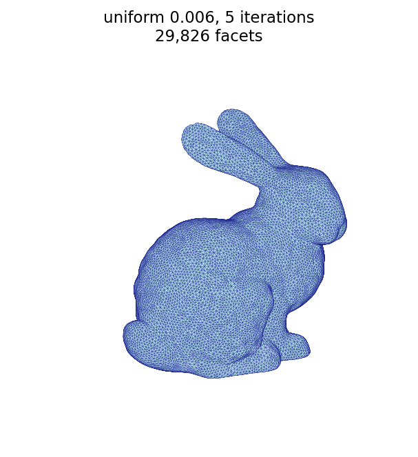 | |
This is the opposite regime from the sphere, where the input was already near the
target and five iterations sufficed. When coarsening a dense scan, increase
--iterations.
Uniform vs. adaptive
This is where the bunny differs most from the sphere. Because the bunny's curvature varies, curvature-adaptive sizing produces a visibly different mesh from uniform sizing at the same triangle budget: adaptive keeps small triangles on high-curvature features (ears, head, paws) and enlarges them on the smooth flanks.
A wide edge-length spread (--minimum 0.002 --maximum 0.040) with a low
--tolerance accentuates this: only the highest-curvature regions are refined to
the minimum, while everything smooth relaxes toward the maximum.
The uniform and adaptive remesh commands
automesh remesh -i stanford_bunny.stl -o bunny_compare_uniform.stl uniform  -s 0.0036 -n 20
automesh remesh -i stanford_bunny.stl -o bunny_adaptive.stl        adaptive --minimum 0.002 --maximum 0.040 -n 25 -t 0.02
| uniform (9,541 facets) | adaptive (9,698 facets) |
|---|---|
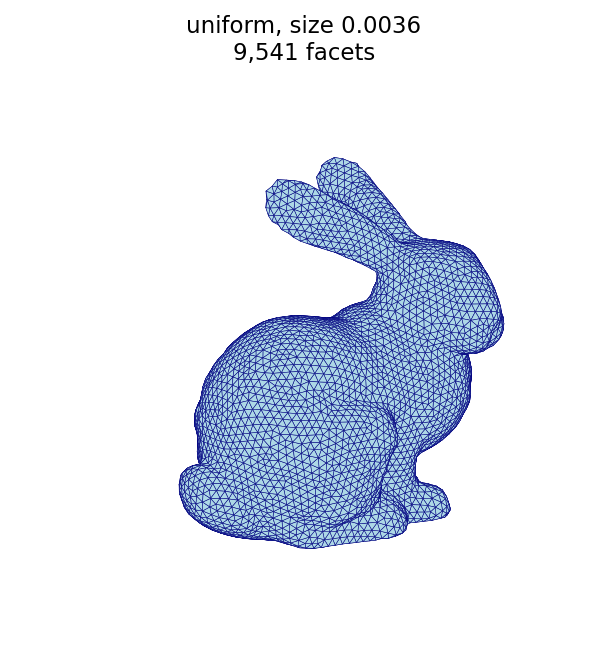 | 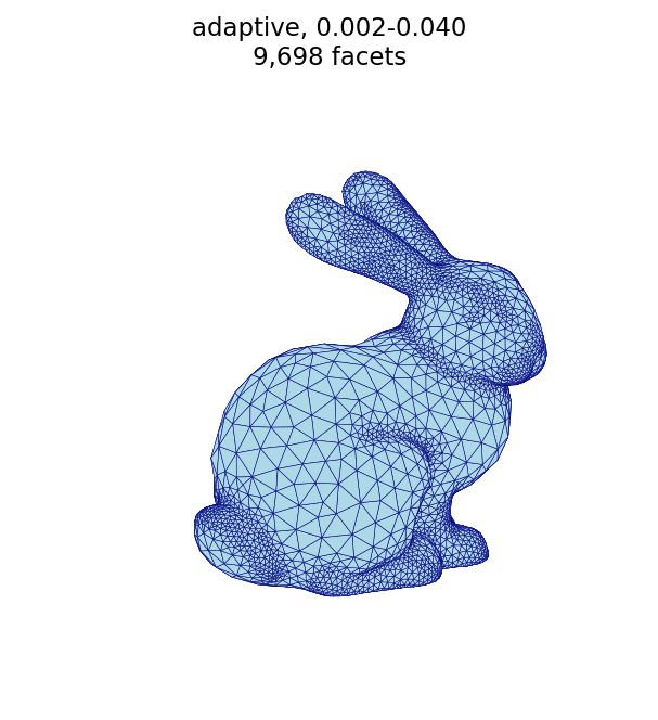 |
Both meshes use a similar number of facets, but adaptive spends them where the surface bends most: the ears, head, and paws are finely triangulated while the smooth flanks and haunches are left coarse.
Adaptive curvature tolerance (--tolerance)
The tolerance sets the target edge length through the
Dunyach sizing formula1,
as implemented in the conspire Rust
library2 on which automesh is
built:
where is the tolerance and is the local surface curvature (flat regions, , take the maximum edge length).
Its effect on the facet count is not monotonic — and this is the part that is
easy to get backwards. Sweeping the tolerance at fixed
--minimum 0.002 --maximum 0.040 -n 25 gives a U-shaped curve:
The three tolerance remesh commands
automesh remesh -i stanford_bunny.stl -o bunny_tol_tight.stl adaptive --minimum 0.002 --maximum 0.040 -n 25 -t 0.0002
automesh remesh -i stanford_bunny.stl -o bunny_tol_mid.stl   adaptive --minimum 0.002 --maximum 0.040 -n 25 -t 0.002
automesh remesh -i stanford_bunny.stl -o bunny_tol_loose.stl adaptive --minimum 0.002 --maximum 0.040 -n 25 -t 0.02
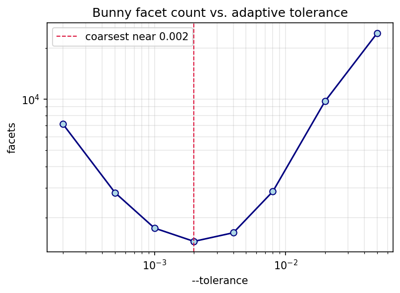
Both very small and very large tolerances refine the mesh; the coarsest result is in between (near here):
tight, -t 0.0002 (7,133 facets) | moderate, -t 0.002 (1,452 facets) | loose, -t 0.02 (9,698 facets) |
|---|---|---|
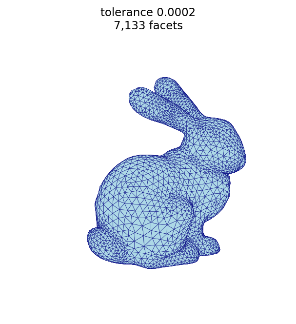 | 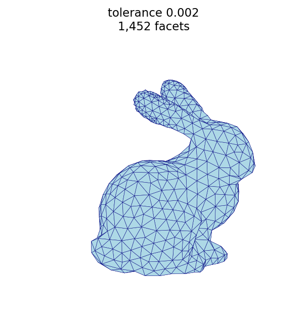 | 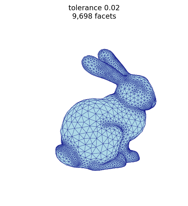 |
Why the U shape? The tolerance acts as a curvature cutoff : regions sharper than clamp to the minimum edge length, while flatter regions follow the formula above.
- Small (large cutoff): few regions reach the cutoff, but the formula itself returns short edges wherever curvature is nonzero, so the mesh is fine.
- Large (small cutoff): the term drives the argument negative over more of the surface, so more regions clamp to the minimum — the mesh is fine again.
- In between, most of the surface sits in the formula regime at moderate edge lengths, giving the coarsest mesh.
In practice, sweep the tolerance for your surface (as above), pick a value near
the coarse minimum, and set --minimum/--maximum for the resolution you want.
The sweep is produced by the
remesh_bunny_tolerance.py script.
Adaptive size gradation (--gradation)
The gradation limits how quickly the target edge length may change between
neighboring triangles. A small gradation forces a slow, smooth transition, so
the fine triangles near features spread outward across the surface (many more
facets); a large gradation allows a rapid transition, keeping the refinement
localized to the features (fewer facets). Using the same baseline as above
(--minimum 0.002 --maximum 0.040 -n 25 -t 0.02):
The two gradation remesh commands
automesh remesh -i stanford_bunny.stl -o bunny_adapt_grad_lo.stl adaptive --minimum 0.002 --maximum 0.040 -n 25 -t 0.02 -g 0.1
automesh remesh -i stanford_bunny.stl -o bunny_adapt_grad_hi.stl adaptive --minimum 0.002 --maximum 0.040 -n 25 -t 0.02 -g 0.9
-g 0.1 — gradual (22,086 facets) | -g 0.9 — sharp (7,016 facets) |
|---|---|
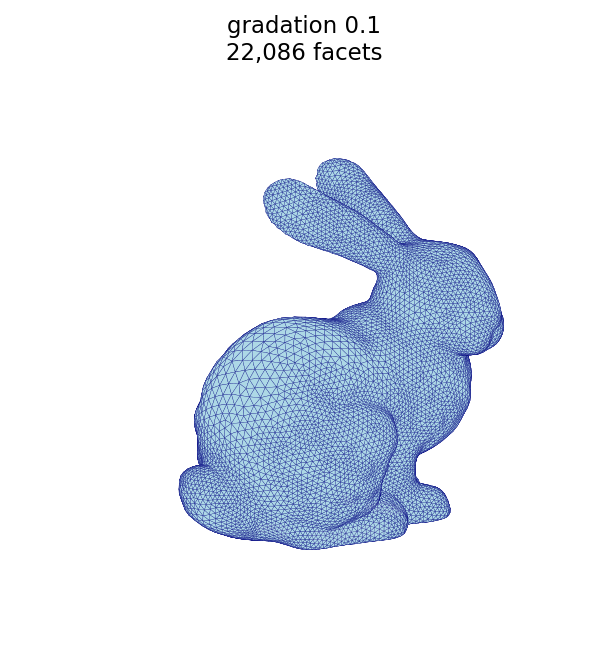 | 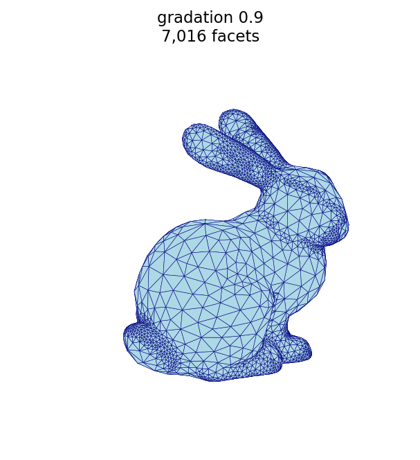 |
Parameters at a glance
| parameter | mode | effect |
|---|---|---|
--size | uniform | target edge length; smaller → more, smaller triangles |
--iterations | both | number of passes; more passes are needed to reach a coarse target from a dense input |
--minimum / --maximum | adaptive | bounds on edge length across the surface |
--tolerance | adaptive | curvature cutoff in the Dunyach formula; facet count is non-monotonic (coarsest at a mid-range value) |
--gradation | adaptive | rate the edge length may change between neighbors; smaller → more gradual (more facets), larger → sharper (fewer facets) |
Figure script
The figures on this page are produced by the following script, which reads each
STL surface and renders it with a matched camera (remapping the bunny's +y
up-axis so it stands upright).
remesh_bunny_figures.py
r"""This module, remesh_bunny_figures.py, renders the Stanford bunny surface
triangulations used in the Stanford bunny remeshing example.  It reads the input
bunny and each remeshed output (produced by `automesh remesh`) and saves a
matched-camera PNG of every mesh.

The bunny's up-axis is +y; the renderer remaps model coordinates (x, y, z) to
plot coordinates (x, z, y) so the bunny stands upright.

Example
-------
source ~/autotwin/automesh/.venv/bin/activate
cd ~/autotwin/automesh/book/examples/remesh
python remesh_bunny_figures.py

Output
------
The `bunny_*.png` visualization files, written next to this script.
"""

import struct
from pathlib import Path
from typing import Final

import matplotlib.pyplot as plt
from mpl_toolkits.mplot3d.art3d import Poly3DCollection
import numpy as np
from numpy.typing import NDArray

# Shared "hero" view so only the triangulation changes between figures.
ELEV: Final[float] = 18.0
AZIM: Final[float] = 55.0
FACECOLOR: Final[str] = "lightblue"
EDGECOLOR: Final[str] = "navy"


def read_stl(path: Path) -> NDArray[np.float64]:
    """Reads triangular facets from a binary STL file, shape (n_facets, 3, 3)."""
    data = path.read_bytes()
    (n_facets,) = struct.unpack_from("<I", data, 80)
    facets = np.empty((n_facets, 3, 3), dtype=np.float64)
    offset = 84
    for i in range(n_facets):
        values = struct.unpack_from("<12f", data, offset)
        facets[i] = np.array(values[3:12]).reshape(3, 3)
        offset += 50
    # Remap (x, y, z) -> (x, z, y) so the bunny's +y up-axis points up in the plot.
    return facets[:, :, [0, 2, 1]]


def edge_lengths(facets: NDArray[np.float64]) -> NDArray[np.float64]:
    """Returns the length of every unique undirected edge in the mesh."""
    keyed = np.round(facets.reshape(-1, 3), 8)
    _, inverse = np.unique(keyed, axis=0, return_inverse=True)
    ids = inverse.reshape(len(facets), 3)
    seen = set()
    lengths = []
    for tri, (a, b, c) in zip(facets, ids):
        for (u, v), (p, q) in (((a, b), (0, 1)), ((b, c), (1, 2)), ((c, a), (2, 0))):
            key = (int(min(u, v)), int(max(u, v)))
            if key not in seen:
                seen.add(key)
                lengths.append(float(np.linalg.norm(tri[p] - tri[q])))
    return np.array(lengths)


def render_histogram(stl: Path, out_name: str) -> None:
    """Saves a histogram of the triangle edge lengths of the given mesh."""
    lengths = edge_lengths(read_stl(stl))
    fig, ax = plt.subplots(figsize=(6, 4))
    ax.hist(lengths, bins=40, color=FACECOLOR, edgecolor=EDGECOLOR)
    ax.axvline(
        lengths.mean(),
        color="crimson",
        linestyle="--",
        linewidth=1.5,
        label=f"mean = {lengths.mean():.4f}",
    )
    ax.set_xlabel("triangle edge length")
    ax.set_ylabel("count")
    ax.set_title(f"{stl.stem}: edge length distribution")
    ax.legend()
    png = stl.with_name(out_name)
    fig.savefig(png, dpi=150, bbox_inches="tight")
    plt.close(fig)
    print(f"wrote {png.name} ({len(lengths):,} edges)")


def render(stl: Path, title: str) -> None:
    """Renders a single bunny STL to a PNG next to it.  Dense meshes are drawn
    without edges (a shaded surface); coarse meshes show their triangle edges."""
    facets = read_stl(stl)
    n = len(facets)
    # Show triangle edges for all but the very dense input scan, which is drawn
    # as a shaded surface.  Thin the lines as the facet count grows.
    show_edges = n <= 40000
    linewidth = 0.25 if n <= 10000 else 0.12
    fig = plt.figure(figsize=(5, 5))
    ax = fig.add_subplot(111, projection="3d")
    surface = Poly3DCollection(
        facets,
        facecolor=FACECOLOR,
        edgecolor=EDGECOLOR if show_edges else "none",
        linewidths=linewidth if show_edges else 0.0,
        rasterized=True,
    )
    surface.set_alpha(1.0)
    ax.add_collection3d(surface)

    pts = facets.reshape(-1, 3)
    lo, hi = pts.min(0), pts.max(0)
    center = (lo + hi) / 2
    radius = (hi - lo).max() / 2
    for setter, c in zip((ax.set_xlim, ax.set_ylim, ax.set_zlim), center):
        setter(c - radius, c + radius)
    ax.set_box_aspect((1, 1, 1))
    ax.view_init(elev=ELEV, azim=AZIM)
    ax.set_axis_off()
    ax.set_title(f"{title}\n{n:,} facets", fontsize=11)
    png = stl.with_suffix(".png")
    fig.savefig(png, dpi=150, bbox_inches="tight")
    plt.close(fig)
    print(f"wrote {png.name} ({n:,} facets)")


def main() -> None:
    here = Path(__file__).resolve().parent
    figures = {
        "stanford_bunny": "input scan",
        "bunny_uniform_fine": "uniform, size 0.004",
        "bunny_uniform_coarse": "uniform, size 0.006",
        "bunny_iter_n5": "uniform 0.006, 5 iterations",
        "bunny_compare_uniform": "uniform, size 0.0036",
        "bunny_adaptive": "adaptive, 0.002-0.040",
        "bunny_tol_tight": "tolerance 0.0002",
        "bunny_tol_mid": "tolerance 0.002",
        "bunny_tol_loose": "tolerance 0.02",
        "bunny_adapt_grad_lo": "adaptive, gradation 0.1",
        "bunny_adapt_grad_hi": "adaptive, gradation 0.9",
    }
    for stem, title in figures.items():
        stl = here / f"{stem}.stl"
        if stl.exists():
            render(stl, title)
        else:
            print(f"skipping {stl.name} (not found)")

    # Edge-length histogram of the input scan.
    base = here / "stanford_bunny.stl"
    if base.exists():
        render_histogram(base, "bunny_edge_histogram.png")


if __name__ == "__main__":
    main()
Tolerance study script
The tolerance sweep plot is produced
by the following script, which remeshes the bunny at several --tolerance values
and records the facet count:
remesh_bunny_tolerance.py
r"""This module, remesh_bunny_tolerance.py, studies how the adaptive
`--tolerance` affects the facet count of the remeshed Stanford bunny.

The adaptive edge length follows the Dunyach formula
``L = sqrt(6 * tolerance / curvature - 3 * tolerance**2)`` clamped to
``[minimum, maximum]``.  Because of the ``- 3 * tolerance**2`` term, the facet
count is *non-monotonic* in the tolerance: very small and very large tolerances
both refine the mesh, with the coarsest result in between.  This script sweeps
the tolerance at fixed ``--minimum``/``--maximum``/``--iterations`` and plots the
resulting facet count.

Example
-------
source ~/autotwin/automesh/.venv/bin/activate
cd ~/autotwin/automesh/book/examples/remesh
# `automesh` must be on the PATH (e.g. target/release)
python remesh_bunny_tolerance.py

Output
------
The `bunny_tolerance.png` plot, written next to this script, and a summary table
printed to the terminal.
"""

import os
import shutil
import struct
import subprocess
import tempfile
from pathlib import Path

import matplotlib.pyplot as plt

TOLERANCES = [0.0002, 0.0005, 0.001, 0.002, 0.004, 0.008, 0.02, 0.05]
MINIMUM, MAXIMUM, ITERATIONS = 0.002, 0.040, 25
FACECOLOR = "lightblue"
EDGECOLOR = "navy"


def automesh_binary() -> str:
    """Locates the `automesh` executable: the AUTOMESH environment variable, then
    the PATH, then the repository's target/release build."""
    candidate = os.environ.get("AUTOMESH") or shutil.which("automesh")
    if candidate:
        return candidate
    fallback = Path(__file__).resolve().parents[2] / "target" / "release" / "automesh"
    if fallback.exists():
        return str(fallback)
    raise FileNotFoundError(
        "could not find `automesh`; set AUTOMESH or add it to the PATH"
    )


def facet_count(stl: Path) -> int:
    """Reads the facet count from a binary STL header (bytes 80-84)."""
    with stl.open("rb") as file:
        file.seek(80)
        return struct.unpack("<I", file.read(4))[0]


def main() -> None:
    here = Path(__file__).resolve().parent
    source = here / "stanford_bunny.stl"
    automesh = automesh_binary()
    counts = []
    print(f"{'tolerance':>10} {'facets':>8}")
    with tempfile.TemporaryDirectory() as tmp:
        for tol in TOLERANCES:
            out = Path(tmp) / "t.stl"
            subprocess.run(
                [automesh, "remesh", "-i", str(source), "-o", str(out),
                 "adaptive", "--minimum", str(MINIMUM), "--maximum", str(MAXIMUM),
                 "-n", str(ITERATIONS), "-t", str(tol)],
                check=True, capture_output=True,
            )
            n = facet_count(out)
            counts.append(n)
            print(f"{tol:>10} {n:>8}")

    coarsest = TOLERANCES[counts.index(min(counts))]
    fig, ax = plt.subplots(figsize=(6, 4))
    ax.plot(TOLERANCES, counts, "o-", color=EDGECOLOR, markerfacecolor=FACECOLOR)
    ax.set_xscale("log")
    ax.set_yscale("log")
    ax.set_xlabel("--tolerance")
    ax.set_ylabel("facets")
    ax.set_title("Bunny facet count vs. adaptive tolerance")
    ax.axvline(
        coarsest, color="crimson", linestyle="--", linewidth=1.0,
        label=f"coarsest near {coarsest}",
    )
    ax.legend()
    ax.grid(True, which="both", alpha=0.3)
    png = here / "bunny_tolerance.png"
    fig.savefig(png, dpi=150, bbox_inches="tight")
    plt.close(fig)
    print(f"wrote {png.name}")


if __name__ == "__main__":
    main()
Helper: OBJ to binary STL
The Stanford bunny is distributed as an OBJ, but remesh reads STL, not OBJ.
This helper converts the downloaded OBJ to the stanford_bunny.stl used above:
obj_to_binary_stl.py
r"""This module, obj_to_binary_stl.py, converts a triangular OBJ mesh into a
binary STL file.  `automesh remesh` reads STL, not OBJ, so the Stanford
bunny OBJ from Alec Jacobson's repository must be converted before use.

Example
-------
source ~/autotwin/automesh/.venv/bin/activate
cd ~/autotwin/automesh/book/examples/remesh
python obj_to_binary_stl.py stanford-bunny.obj stanford_bunny.stl
"""

import struct
import sys
from pathlib import Path

import numpy as np


def obj_to_binary_stl(source: Path, target: Path) -> None:
    """Reads a triangular OBJ and writes an equivalent binary STL."""
    verts: list[tuple[float, float, float]] = []
    faces: list[tuple[int, int, int]] = []
    for line in source.read_text().splitlines():
        tokens = line.split()
        if not tokens:
            continue
        if tokens[0] == "v":
            verts.append(tuple(float(x) for x in tokens[1:4]))
        elif tokens[0] == "f":
            # OBJ is 1-indexed; entries may be v, v/vt, or v/vt/vn. Fan-triangulate.
            idx = [int(p.split("/")[0]) - 1 for p in tokens[1:]]
            for k in range(1, len(idx) - 1):
                faces.append((idx[0], idx[k], idx[k + 1]))

    coords = np.array(verts, dtype=np.float64)
    with target.open("wb") as out:
        out.write(b"\0" * 80)  # 80-byte header (ignored)
        out.write(struct.pack("<I", len(faces)))  # facet count
        for a, b, c in faces:
            p, q, r = coords[a], coords[b], coords[c]
            normal = np.cross(q - p, r - p)
            length = np.linalg.norm(normal)
            normal = normal / length if length > 0 else normal
            out.write(struct.pack("<12fH", *normal, *p, *q, *r, 0))
    print(f"wrote {len(faces)} facets to {target}")


if __name__ == "__main__":
    if len(sys.argv) != 3:
        sys.exit("usage: python obj_to_binary_stl.py <mesh.obj> <mesh.stl>")
    obj_to_binary_stl(Path(sys.argv[1]), Path(sys.argv[2]))
References
-
Dunyach M, Vanderhaeghe D, Barthe L, Botsch M. Adaptive remeshing for real-time mesh deformation. In Eurographics 2013 Short Papers. 2013. paper · DOI ↩
-
Buche MR. conspire — a Rust library for computational continuum mechanics, version 0.7.3. repository · crate ↩
Mesh example: Remeshed Unit Sphere
The Torus example builds an all-hexahedral mesh directly from a
segmentation, one hexahedron per voxel. Here we take the other route into
mesh hex: its tessellation input. Given a triangular surface mesh,
mesh hex fills the enclosed volume with hexahedra by octree dualization.
The surface we start from is the remeshed unit sphere from the
Remesh: Unit Sphere example — specifically its -n 10
output, a clean, near-uniform triangulation of 856 facets. This example
turns that triangular surface into a solid all-hexahedral volume.
Downloadable Files
| file | description |
|---|---|
| sphere_n10.stl | The remeshed triangular sphere surface (856 facets), the input to dualization (see Preparing the Surface). |
| sphere_hex.inp | The all-hexahedral mesh produced from it (see Dualizing to Hexahedra). |
Preparing the Surface
sphere_n10.stl is reproduced here by running the -n 10 uniform remesh
from the Remesh: Unit Sphere example on its
sphere_radius_1.stl input:
The remesh command
automesh remesh -i sphere_radius_1.stl -o sphere_n10.stl uniform -n 10
Dualizing to Hexahedra
mesh hex on a tessellation converts the surface into a solid hexahedral
mesh. The --scale option sets the octree refinement depth — how finely
the bounding box is subdivided before the surface is captured:
The mesh hex command and output
automesh mesh hex -i sphere_n10.stl -o sphere_hex.inp --scale 8
    automesh 0.5.1
     Reading sphere_n10.stl
        Done 173.813µs
     Meshing hexahedra adaptively
        Done 13.005419ms [203 elements, 360 nodes]
   Buffering hexahedra onto geometry
        Done 375.978306ms [473 elements, 632 nodes]
     Writing sphere_hex.inp
        Done 349.189µs
       Total 390.105002ms
| triangular surface (856 facets) | all-hexahedral (393 elements) |
|---|---|
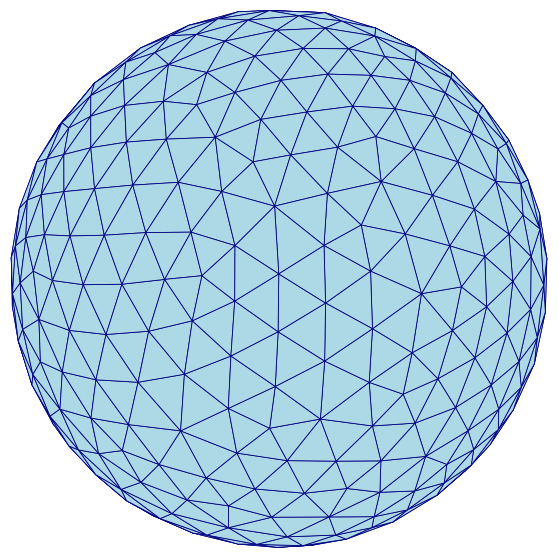 | 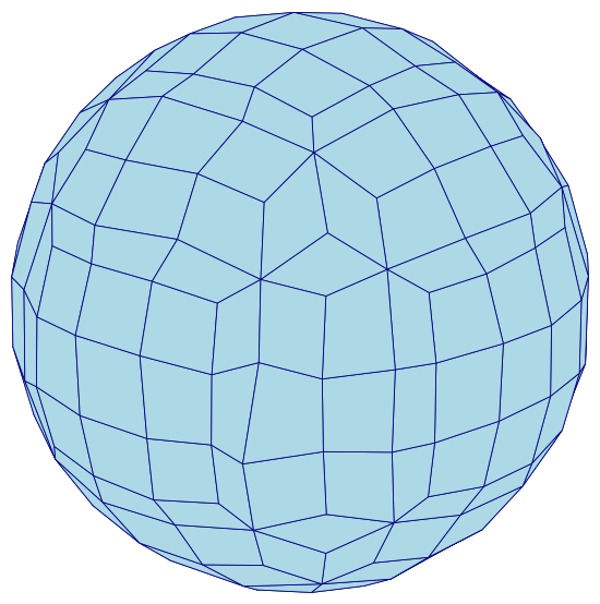 |
Figure 4.7-1: The remeshed triangular surface (left) and the solid all-hexahedral volume dualized from it (right). The surface only bounds the sphere; the hex mesh fills its interior.
Choosing --scale
Unlike the segmentation route, the tessellation route does not have a
natural element size baked into the input, so --scale matters — and its
effect on element quality is not monotonic. Sweeping it, and checking
the minimum scaled Jacobian with metrics, gives:
--scale | elements | min scaled Jacobian | mean scaled Jacobian |
|---|---|---|---|
| 3 (default) | 7 | — | — |
| 6 | 183 | 0.058 | 0.633 |
| 7 | 235 | 0.058 | 0.728 |
| 8 | 393 | 0.280 | 0.766 |
| 9 | 551 | 0.009 | 0.783 |
| 10 | 804 | -0.165 | 0.772 |
At the default --scale 3, the octree barely subdivides this small
(radius ≈ 1) bounding box, giving just 7 elements — far too coarse for a
sphere. Increasing --scale refines the mesh, but pushing it too far is
counterproductive: at --scale 9 the worst element drops back toward zero,
and at --scale 10 the mesh contains inverted elements (negative scaled
Jacobian), where the octree grid meets the curved surface at an
irrecoverable angle.
--scale 8 is the sweet spot for this sphere: 393 well-formed elements with
a minimum scaled Jacobian of 0.280 and no inverted elements. The right
value is geometry-dependent, so sweep it and check metrics, rather than
simply raising it until the mesh looks fine.
Element Quality
The --scale 8 mesh, evaluated with metrics:
| metric | min | mean | max |
|---|---|---|---|
| minimum scaled Jacobian | 0.280 | 0.766 | 1.000 |
| maximum skew | 0.000 | 0.202 | 0.680 |
| maximum edge ratio | 1.000 | 1.745 | 3.306 |
Unlike the Torus's raw voxel mesh — where every element starts as
a perfect unit cube — a dualized mesh never has trivially perfect elements:
the octree cells must deform to conform to the curved surface. The worst
element here (scaled Jacobian 0.280) sits where a coarse octree cell meets
the sphere; it is still an acceptable element, but it is the reason the
--scale sweep above is worth doing.
Source
The figures on this page are produced by the following script, which reads
the triangular surface (sphere_n10.stl) and the hexahedral mesh
(sphere_hex.inp, extracting its exterior quad faces) and renders both with
a matched camera:
sphere_hex_figures.py
r"""This module, sphere_hex_figures.py, renders the remeshed triangular
sphere surface and the all-hexahedral mesh produced from it by octree
dualization, used in the remeshed unit sphere mesh example.

Example
-------
source ~/autotwin/automesh/.venv/bin/activate
cd ~/autotwin/automesh/book/examples/mesh
automesh remesh -i ../remesh/sphere_radius_1.stl -o sphere_n10.stl uniform -n 10
automesh mesh hex -i sphere_n10.stl -o sphere_hex.inp --scale 8
python sphere_hex_figures.py

Output
------
The `sphere_tri.png` and `sphere_hex.png` visualization files, written next
to this script.
"""

import struct
from collections import Counter
from pathlib import Path
from typing import Final

import matplotlib.pyplot as plt
from mpl_toolkits.mplot3d.art3d import Poly3DCollection
import numpy as np
from numpy.typing import NDArray
from PIL import Image

# Shared "hero" view so only the mesh changes between figures.
ELEV: Final[float] = 22.0
AZIM: Final[float] = -50.0
FACECOLOR: Final[str] = "lightblue"
EDGECOLOR: Final[str] = "navy"

# Local (0-indexed) face node order for an Abaqus C3D8 hexahedron.
C3D8_FACES: Final[tuple[tuple[int, int, int, int], ...]] = (
    (0, 1, 2, 3),
    (4, 5, 6, 7),
    (0, 1, 5, 4),
    (1, 2, 6, 5),
    (2, 3, 7, 6),
    (3, 0, 4, 7),
)


def read_stl(path: Path) -> NDArray[np.float64]:
    """Reads triangular facets from a binary STL file, shape (n_facets, 3, 3)."""
    data = path.read_bytes()
    (n_facets,) = struct.unpack_from("<I", data, 80)
    facets = np.empty((n_facets, 3, 3), dtype=np.float64)
    offset = 84
    for i in range(n_facets):
        values = struct.unpack_from("<12f", data, offset)
        facets[i] = np.array(values[3:12]).reshape(3, 3)
        offset += 50
    return facets


def read_inp_hex(
    path: Path,
) -> tuple[dict[int, tuple[float, float, float]], list[tuple[int, ...]]]:
    """Reads nodes and C3D8 element connectivity from an Abaqus .inp file."""
    nodes: dict[int, tuple[float, float, float]] = {}
    elements: list[tuple[int, ...]] = []
    section = None
    for line in path.read_text().splitlines():
        stripped = line.strip()
        if not stripped:
            continue
        if stripped.startswith("*"):
            lower = stripped.lower()
            section = (
                "node"
                if lower.startswith("*node")
                else "element"
                if lower.startswith("*element")
                else None
            )
            continue
        parts = [p.strip() for p in stripped.split(",")]
        if section == "node":
            nodes[int(parts[0])] = tuple(float(v) for v in parts[1:4])
        elif section == "element":
            ids = [int(p) for p in parts]
            elements.append(tuple(ids[1:9]))
    return nodes, elements


def exterior_quads(
    nodes: dict[int, tuple[float, float, float]],
    elements: list[tuple[int, ...]],
) -> list[NDArray[np.float64]]:
    """Returns the mesh's exterior quad faces, each as a (4, 3) coordinate
    array.  A face is exterior if it belongs to exactly one hex element."""
    face_count: Counter[frozenset[int]] = Counter()
    for elem in elements:
        for face in C3D8_FACES:
            face_count[frozenset(elem[i] for i in face)] += 1

    quads = []
    seen: set[frozenset[int]] = set()
    for elem in elements:
        for face in C3D8_FACES:
            node_ids = tuple(elem[i] for i in face)
            key = frozenset(node_ids)
            if face_count[key] == 1 and key not in seen:
                seen.add(key)
                quads.append(np.array([nodes[n] for n in node_ids]))
    return quads


def crop_to_content(path: Path, margin: int = 10) -> None:
    """Crops a saved PNG to its non-white content, since matplotlib's
    `bbox_inches="tight"` does not shrink the whitespace 3D axes leave
    around a plot even with the axes turned off."""
    image = Image.open(path).convert("RGB")
    array = np.asarray(image)
    non_white = np.any(array != 255, axis=-1)
    rows = np.where(non_white.any(axis=1))[0]
    cols = np.where(non_white.any(axis=0))[0]
    top = max(rows.min() - margin, 0)
    bottom = min(rows.max() + margin + 1, array.shape[0])
    left = max(cols.min() - margin, 0)
    right = min(cols.max() + margin + 1, array.shape[1])
    image.crop((left, top, right, bottom)).save(path)


def render_faces(
    faces: list[NDArray[np.float64]],
    bounds: tuple[NDArray[np.float64], NDArray[np.float64]],
    out_path: Path,
) -> None:
    """Renders a list of polygon faces (triangles or quads) as a shaded 3D
    surface, framed to the given (mins, maxs) bounds so companion figures
    share an identical scale."""
    mins, maxs = bounds
    fig = plt.figure(figsize=(6, 6))
    ax = fig.add_subplot(projection="3d")
    ax.add_collection3d(
        Poly3DCollection(faces, facecolor=FACECOLOR, edgecolor=EDGECOLOR, linewidths=0.4)
    )
    ax.set_xlim(mins[0], maxs[0])
    ax.set_ylim(mins[1], maxs[1])
    ax.set_zlim(mins[2], maxs[2])
    ax.set_box_aspect(tuple(maxs - mins))
    ax.view_init(elev=ELEV, azim=AZIM)
    ax.set_axis_off()
    fig.subplots_adjust(left=0, right=1, bottom=0, top=1)
    fig.savefig(out_path, dpi=150, bbox_inches="tight", pad_inches=0.02)
    plt.close(fig)
    crop_to_content(out_path)
    print(f"wrote {out_path} ({len(faces)} faces)")


if __name__ == "__main__":
    triangles = [f for f in read_stl(Path("sphere_n10.stl"))]

    nodes, elements = read_inp_hex(Path("sphere_hex.inp"))
    quads = exterior_quads(nodes, elements)

    # Share one reference bounding box (the union of both meshes' extents) so
    # the triangular surface and the hex mesh render at an identical scale.
    all_points = np.concatenate([np.concatenate(triangles), np.concatenate(quads)])
    bounds = (all_points.min(axis=0), all_points.max(axis=0))

    render_faces(triangles, bounds, Path("sphere_tri.png"))
    render_faces(quads, bounds, Path("sphere_hex.png"))
Laplace Smoothing
Double X
We examine the most basic type of smoothing, Laplace smoothing, , without hierarchical control, with the Double X example.

Figure 4.8-1: The Double X two-element example.
Table. The neighborhoods table. A node, with its neighbors, is considered a single neighborhood. The table has twelve neighborhoods.
| node | node neighbors |
|---|---|
| 1 | 2, 4, 7 |
| 2 | 1, 3, 5, 8 |
| 3 | 2, 6, 9 |
| 4 | 1, 5, 10 |
| 5 | 2, 4, 6, 11 |
| 6 | 3, 5, 12 |
| 7 | 1, 8, 10 |
| 8 | 2, 7, 9, 11 |
| 9 | 3, 8, 12 |
| 10 | 4, 7, 11 |
| 11 | 5, 8, 10, 12 |
| 12 | 6, 9, 11 |
Hierarchy
Following is a test where all nodes are BOUNDARY from the Hierarchy enum.
node_hierarchy: NodeHierarchy = (
    Hierarchy.BOUNDARY,
    Hierarchy.BOUNDARY,
    Hierarchy.BOUNDARY,
    Hierarchy.BOUNDARY,
    Hierarchy.BOUNDARY,
    Hierarchy.BOUNDARY,
    Hierarchy.BOUNDARY,
    Hierarchy.BOUNDARY,
    Hierarchy.BOUNDARY,
    Hierarchy.BOUNDARY,
    Hierarchy.BOUNDARY,
    Hierarchy.BOUNDARY,
)
Since there are no
INTERIORnodes norPRESCRIBEDnodes, the effect of hierarchical smoothing is nil, and the same effect would be observed were all nodes categorized asINTERIORnodes.
Iteration 1
Table: The smoothed configuration (x, y, z) after one iteration of Laplace smoothing.
| node | x | y | z |
|---|---|---|---|
| 1 | 0.1 | 0.1 | 0.1 |
| 2 | 1.0 | 0.075 | 0.075 |
| 3 | 1.9 | 0.1 | 0.1 |
| 4 | 0.1 | 0.9 | 0.1 |
| 5 | 1.0 | 0.925 | 0.075 |
| 6 | 1.9 | 0.9 | 0.1 |
| 7 | 0.1 | 0.1 | 0.9 |
| 8 | 1.0 | 0.075 | 0.925 |
| 9 | 1.9 | 0.1 | 0.9 |
| 10 | 0.1 | 0.9 | 0.9 |
| 11 | 1.0 | 0.925 | 0.925 |
| 12 | 1.9 | 0.9 | 0.9 |
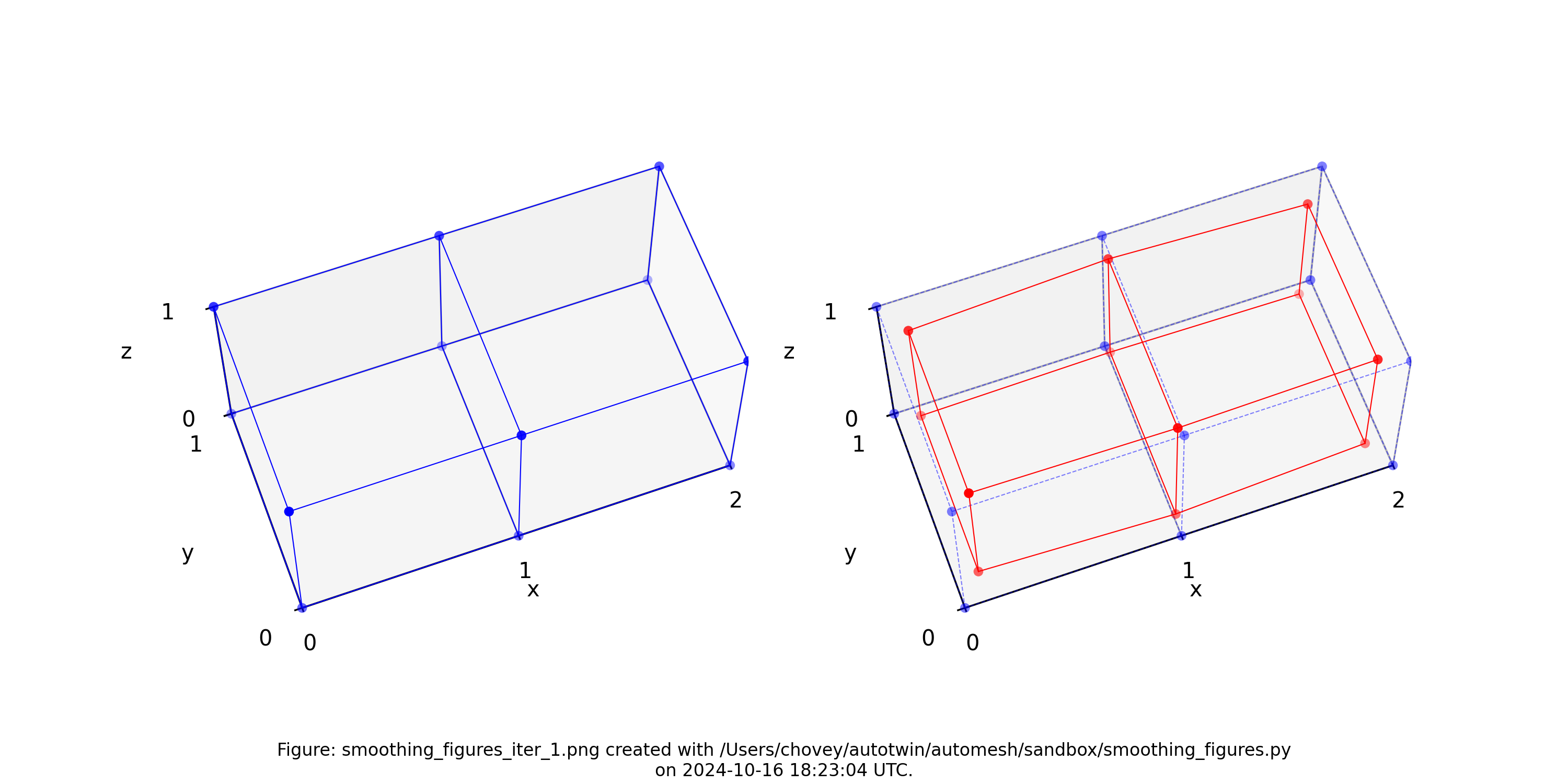
Figure 4.8-2: Two element test problem (left) original configuration, (right) subject to one iteration of Laplace smoothing.
Iteration 2
| node | x | y | z |
|---|---|---|---|
| 1 | 0.19 | 0.1775 | 0.1775 |
| 2 | 1.0 | 0.1425 | 0.1425 |
| 3 | 1.81 | 0.1775 | 0.1775 |
| 4 | 0.19 | 0.8225 | 0.1775 |
| 5 | 1.0 | 0.8575 | 0.1425 |
| 6 | 1.81 | 0.8225 | 0.1775 |
| 7 | 0.19 | 0.1775 | 0.8225 |
| 8 | 1.0 | 0.1425 | 0.8575 |
| 9 | 1.81 | 0.1775 | 0.8225 |
| 10 | 0.19 | 0.8225 | 0.8225 |
| 11 | 1.0 | 0.8575 | 0.8575 |
| 12 | 1.81 | 0.8225 | 0.8225 |
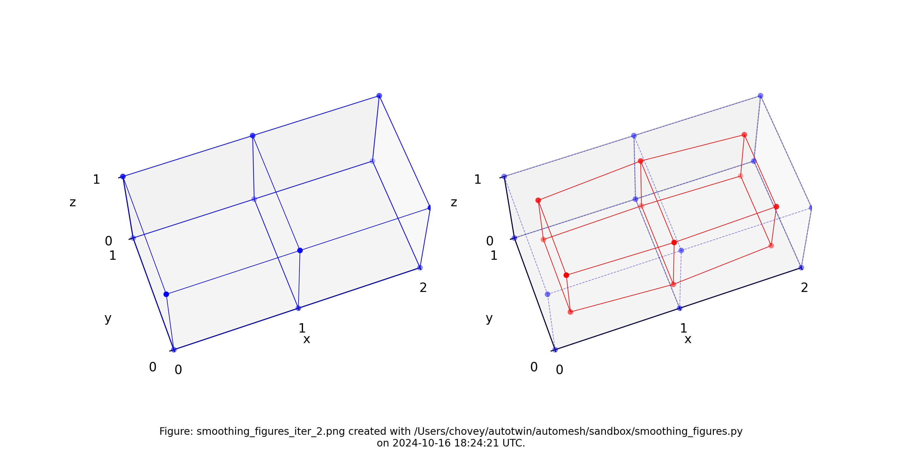
Figure 4.8-3: Two element test problem (left) original configuration, (right) subject to two iterations of Laplace smoothing.
Iteration 100
A known drawback of Laplace smoothing is that it can fail to preserve volumes. In the limit, volumes get reduced to a point, as illustrated in the figure below.
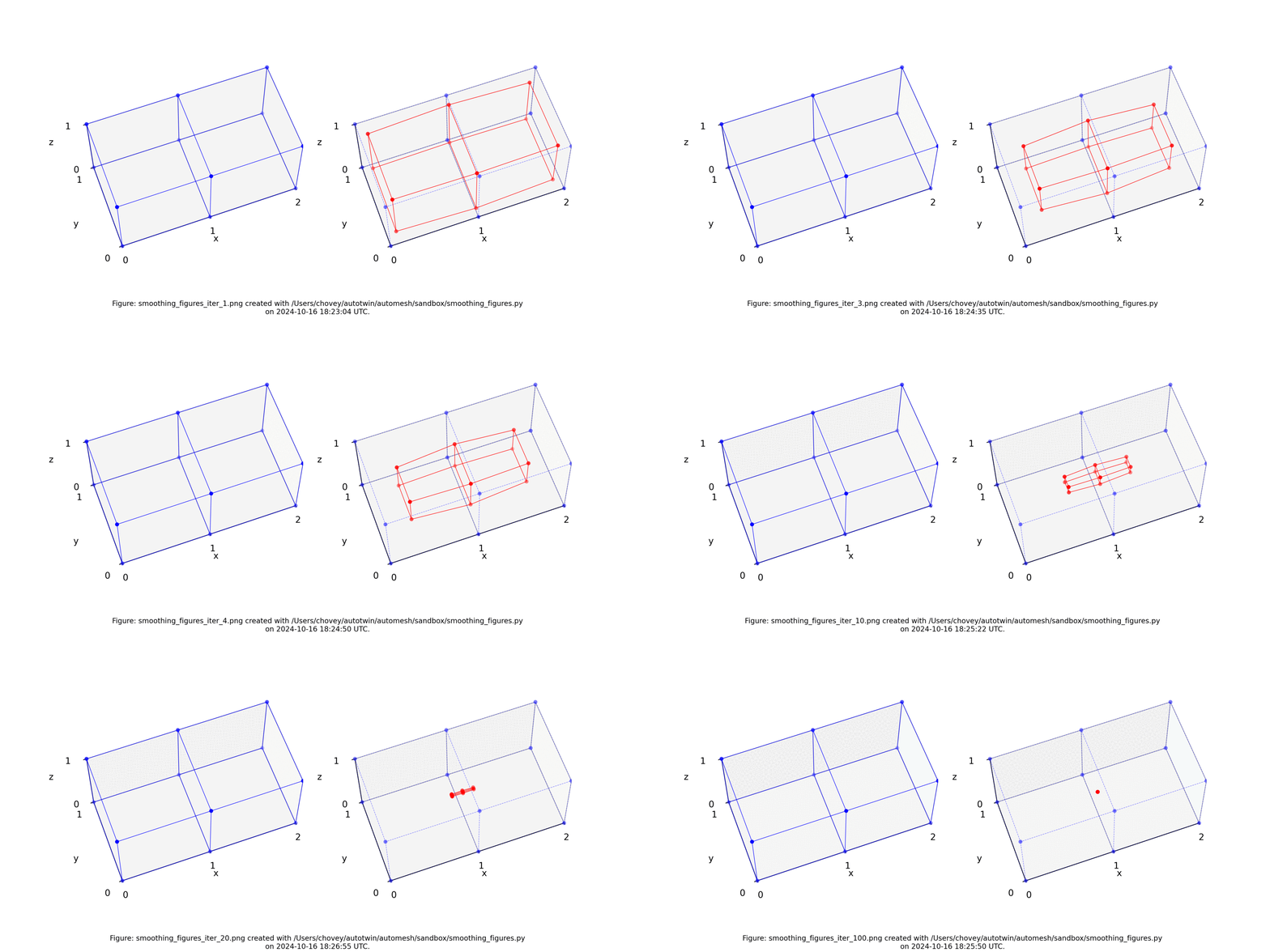
Figure 4.8-4: Two element test problem (left) original configuration, (right) subject to [1, 2, 3, 4, 5, 10, 20, 30, 100 iterations of Laplace smoothing. Animation created with Ezgif.
Laplace Smoothing with Hierarchical Control
Laplace Smoothing, Hierarchical Control, Prescribed Homogeneous
Cube with Inclusion

To come.
Laplace Smoothing, Hierarchical Control, Prescribed Inhomogeneous
Bracket
To begin to examine hierarchical control, we consider the Bracket example.

Figure 4.9-1: The Bracket example.
Laplace Smoothing without Hierarchical Control
As a baseline, let's examine what Laplace smoothing, , without hierarchical control performs.
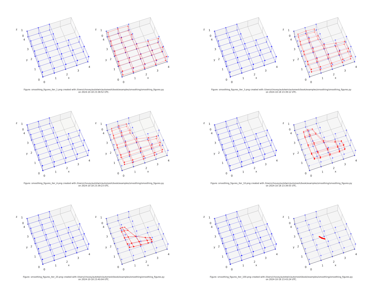
Figure 4.9-2: The Bracket test problem (left) original configuration, (right) subject to [1, 2, 3, 4, 5, 10, 20, 30, 100] iterations of Laplace smoothing. Animation created with Ezgif.
As an example, the nodal positions after 10 iterations are as follows:
| node | x | y | z |
|---|---|---|---|
| 1 | 0.6603416706977089 | 0.6603416706977089 | 0.42058348557613 |
| 2 | 1.164014406316456 | 0.5922705223353653 | 0.4003570849733875 |
| 3 | 1.9979372129260855 | 0.5706936094999626 | 0.39548539946279243 |
| 4 | 2.8325693635137097 | 0.5703120664922405 | 0.40180333889841546 |
| 5 | 3.332396179530681 | 0.6196854057408008 | 0.4228468310236131 |
| 6 | 0.5922705223353653 | 1.164014406316456 | 0.4003570849733875 |
| 7 | 1.129330412354556 | 1.129330412354556 | 0.3779268501553354 |
| 8 | 1.986117815900869 | 1.100245269915641 | 0.3744217105825115 |
| 9 | 2.8536168286772536 | 1.0284532492877596 | 0.3839611664938703 |
| 10 | 3.3805688588919414 | 1.007196857251266 | 0.40846995582593837 |
| 11 | 0.5706936094999626 | 1.9979372129260853 | 0.39548539946279243 |
| 12 | 1.100245269915641 | 1.986117815900869 | 0.37442171058251145 |
| 13 | 1.9089262792820898 | 1.90892627928209 | 0.3766933485101331 |
| 14 | 2.816962753463538 | 1.5457873563122884 | 0.3970154773256839 |
| 15 | 3.3296020281899956 | 1.409074280806729 | 0.42165070606234384 |
| 16 | 0.5703120664922405 | 2.8325693635137097 | 0.40180333889841546 |
| 17 | 1.0284532492877596 | 2.8536168286772536 | 0.3839611664938703 |
| 18 | 1.5457873563122884 | 2.816962753463538 | 0.3970154773256839 |
| 19 | 0.6196854057408008 | 3.332396179530681 | 0.4228468310236131 |
| 20 | 1.007196857251266 | 3.3805688588919414 | 0.40846995582593837 |
| 21 | 1.409074280806729 | 3.3296020281899956 | 0.42165070606234384 |
| 22 | 0.6603416706977089 | 0.6603416706977089 | 0.5794165144238701 |
| 23 | 1.164014406316456 | 0.5922705223353653 | 0.5996429150266126 |
| 24 | 1.9979372129260853 | 0.5706936094999626 | 0.6045146005372077 |
| 25 | 2.8325693635137097 | 0.5703120664922404 | 0.5981966611015848 |
| 26 | 3.332396179530681 | 0.6196854057408007 | 0.5771531689763871 |
| 27 | 0.5922705223353654 | 1.164014406316456 | 0.5996429150266126 |
| 28 | 1.129330412354556 | 1.129330412354556 | 0.6220731498446648 |
| 29 | 1.986117815900869 | 1.100245269915641 | 0.6255782894174887 |
| 30 | 2.8536168286772536 | 1.0284532492877596 | 0.6160388335061299 |
| 31 | 3.3805688588919414 | 1.0071968572512657 | 0.5915300441740619 |
| 32 | 0.5706936094999626 | 1.9979372129260853 | 0.6045146005372076 |
| 33 | 1.100245269915641 | 1.986117815900869 | 0.6255782894174885 |
| 34 | 1.90892627928209 | 1.9089262792820898 | 0.623306651489867 |
| 35 | 2.816962753463538 | 1.5457873563122881 | 0.6029845226743162 |
| 36 | 3.3296020281899956 | 1.409074280806729 | 0.5783492939376563 |
| 37 | 0.5703120664922404 | 2.8325693635137097 | 0.5981966611015848 |
| 38 | 1.0284532492877596 | 2.8536168286772536 | 0.6160388335061298 |
| 39 | 1.5457873563122884 | 2.816962753463538 | 0.6029845226743162 |
| 40 | 0.6196854057408007 | 3.332396179530681 | 0.5771531689763871 |
| 41 | 1.0071968572512657 | 3.3805688588919414 | 0.5915300441740617 |
| 42 | 1.409074280806729 | 3.3296020281899956 | 0.5783492939376562 |
Laplace Smoothing with Hierarchical Control
We illustrate the how hierarchical control affects the Laplace smoothing.
Consider the PRESCRIBED and BOUNDARY node hierarchy below:
node_hierarchy: NodeHierarchy = (
    # hierarchy enum, node number, prescribed (x, y, z)
    Hierarchy.PRESCRIBED,  # 1 -> (0, 0, 0)
    Hierarchy.PRESCRIBED,  # 2 -> (1, 0, 0)
    Hierarchy.PRESCRIBED,  # 3 -> (2, 0, 0)
    Hierarchy.PRESCRIBED,  # 4 -> (3, 0, 0)
    Hierarchy.PRESCRIBED,  # 5 -> (4, 0, 0)
    Hierarchy.PRESCRIBED,  # 6 -> (0, 1, 0)
    Hierarchy.BOUNDARY,  # 7
    Hierarchy.BOUNDARY,  # 8
    Hierarchy.BOUNDARY,  # 9
    Hierarchy.PRESCRIBED,  # 10 -> (4.5*cos(15 deg), 4.5*sin(15 deg), 0)
    Hierarchy.PRESCRIBED,  # 11 -> *(0, 2, 0)
    Hierarchy.BOUNDARY,  # 12
    Hierarchy.BOUNDARY,  # 13
    Hierarchy.BOUNDARY,  # 14
    Hierarchy.PRESCRIBED,  # 15 -> (4.5*cos(30 deg), 4.5*sin(30 deg), 0)
    Hierarchy.PRESCRIBED,  # 16 -> (0, 3, 0)
    Hierarchy.BOUNDARY,  # 17
    Hierarchy.BOUNDARY,  # 18
    Hierarchy.PRESCRIBED,  # 19 -> (0, 4, 0)
    Hierarchy.PRESCRIBED,  # 20 -> (1.5, 4, 0)
    Hierarchy.PRESCRIBED,  # 21 -> (3.5, 4, 0)
    #
    Hierarchy.PRESCRIBED,  # 22 -> (0, 0, 1)
    Hierarchy.PRESCRIBED,  # 23 -> (1, 0, 1)
    Hierarchy.PRESCRIBED,  # 24 -> (2, 0, 1)
    Hierarchy.PRESCRIBED,  # 25 -> (3, 0, 1)
    Hierarchy.PRESCRIBED,  # 26 -> (4, 0, 1)
    Hierarchy.PRESCRIBED,  # 27 -> (0, 1, 1)
    Hierarchy.BOUNDARY,  # 28
    Hierarchy.BOUNDARY,  # 29
    Hierarchy.BOUNDARY,  # 30
    Hierarchy.PRESCRIBED,  # 31 -> (4.5*cos(15 deg), 4.5*sin(15 deg), 1)
    Hierarchy.PRESCRIBED,  # 32 -> *(0, 2, 1)
    Hierarchy.BOUNDARY,  # 33
    Hierarchy.BOUNDARY,  # 34
    Hierarchy.BOUNDARY,  # 35
    Hierarchy.PRESCRIBED,  # 36 -> (4.5*cos(30 deg), 4.5*sin(30 deg), 1)
    Hierarchy.PRESCRIBED,  # 37 -> (0, 3, 1)
    Hierarchy.BOUNDARY,  # 38
    Hierarchy.BOUNDARY,  # 39
    Hierarchy.PRESCRIBED,  # 40 -> (0, 4, 1)
    Hierarchy.PRESCRIBED,  # 41 -> (1.5, 4, 1)
    Hierarchy.PRESCRIBED,  # 42 -> (3.5, 4, 1)
)
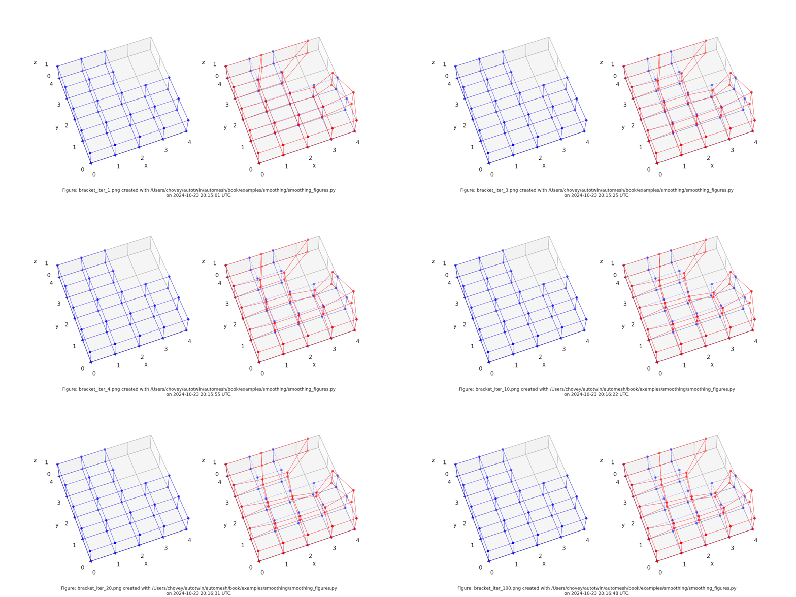
Figure 4.9-3: The Bracket test problem (left) original configuration, (right) subject to [1, 2, 3, 4, 5, 10, 20, 30, 100] iterations of Laplace smoothing with hierarchical control. Animation created with Ezgif.
As an example, the nodal positions after 10 iterations are as follows:
| node | x | y | z |
|---|---|---|---|
| 1 | 0 | 0 | 0 |
| 2 | 1 | 0 | 0 |
| 3 | 2 | 0 | 0 |
| 4 | 3 | 0 | 0 |
| 5 | 4 | 0 | 0 |
| 6 | 0 | 1 | 0 |
| 7 | 1.0076218690550747 | 0.9988829259123082 | 0.24593434133370803 |
| 8 | 2.0218051968023 | 0.993985105791881 | 0.2837944855813176 |
| 9 | 3.0816593568068398 | 0.9931227966186256 | 0.24898414051620496 |
| 10 | 4.346666218300808 | 1.1646857029613433 | 0 |
| 11 | 0 | 2 | 0 |
| 12 | 1.0346002406957664 | 1.992982526945126 | 0.2837944855813176 |
| 13 | 2.0408618916639916 | 1.9528647520642073 | 0.3332231502067546 |
| 14 | 2.9955771790244468 | 1.7619821132207711 | 0.29909606343914835 |
| 15 | 3.897114317029974 | 2.2499999999999996 | 0 |
| 16 | 0 | 3 | 0 |
| 17 | 1.157261281731803 | 2.9982665159532105 | 0.24898414051620493 |
| 18 | 2.1973691292662734 | 2.991054895165017 | 0.29909606343914835 |
| 19 | 0 | 4 | 0 |
| 20 | 1.5 | 4 | 0 |
| 21 | 3.5 | 4 | 0 |
| 22 | 0 | 0 | 1 |
| 23 | 1 | 0 | 1 |
| 24 | 2 | 0 | 1 |
| 25 | 3 | 0 | 1 |
| 26 | 4 | 0 | 1 |
| 27 | 0 | 1 | 1 |
| 28 | 1.0076218690550747 | 0.9988829259123082 | 0.7540656586662919 |
| 29 | 2.0218051968023 | 0.993985105791881 | 0.7162055144186824 |
| 30 | 3.0816593568068398 | 0.9931227966186257 | 0.7510158594837951 |
| 31 | 4.346666218300808 | 1.1646857029613433 | 1 |
| 32 | 0 | 2 | 1 |
| 33 | 1.0346002406957664 | 1.9929825269451262 | 0.7162055144186824 |
| 34 | 2.0408618916639916 | 1.9528647520642073 | 0.6667768497932453 |
| 35 | 2.9955771790244468 | 1.7619821132207711 | 0.7009039365608517 |
| 36 | 3.897114317029974 | 2.2499999999999996 | 1 |
| 37 | 0 | 3 | 1 |
| 38 | 1.157261281731803 | 2.9982665159532105 | 0.751015859483795 |
| 39 | 2.1973691292662734 | 2.991054895165017 | 0.7009039365608516 |
| 40 | 0 | 4 | 1 |
| 41 | 1.5 | 4 | 1 |
| 42 | 3.5 | 4 | 1 |
Taubin Smoothing
We examine the Taubin smoothing algorithm on a sphere composed of hexahedral elements. We created a two block (green inner volume, yellow outer volume) mesh in Cubit, then added normal noise to the hemisphere where the coordinate was positive. We then applied Taubin smoothing to the noised model.
Downloadable Files
The Cubit and Python code used to generate the noised input file and figures
is included below. The .inp mesh files used as input to the
automesh smooth commands in the automesh section — the
original two-material sphere mesh, and the same mesh with normal noise added
to the hemisphere — can be downloaded directly:
| file | size (MB) | md5 checksum |
|---|---|---|
| sphere_res_1cm.inp | 1.5 | 644ef573c257222bfd61dcfda7131c6a |
| sphere_res_1cm_noised.inp | 1.5 | 7031df475b972b15cf28bf2c5b69c162 |
These two files are hosted externally (not in the repository) because of their
size, and are not regenerated automatically as part of the book build. The
smoothed outputs shown below (s10.exo, s50.exo, s200.exo) are likewise
not themselves available for download — only their rendered screenshots are
checked into the repository.
The two-material sphere_res_1cm_noised.inp file is visualized below with and without a midplane cut.
| iso | iso midplane | xz midplane |
|---|---|---|
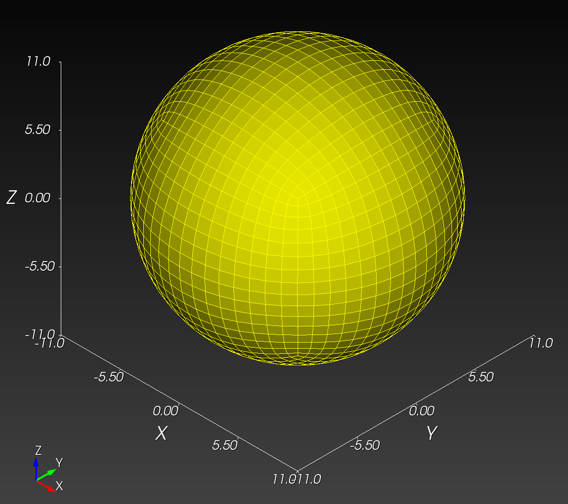 | 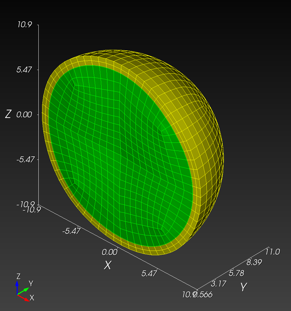 | 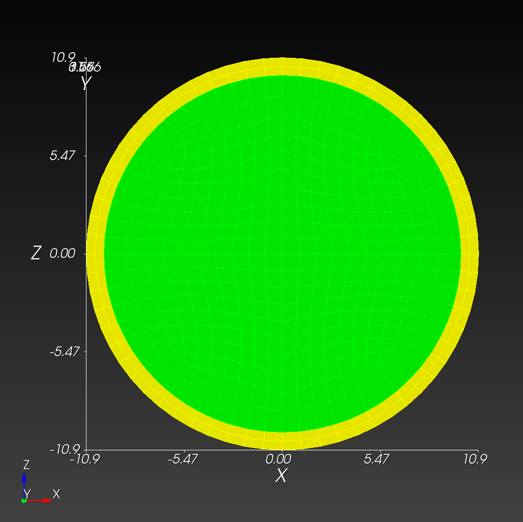 |
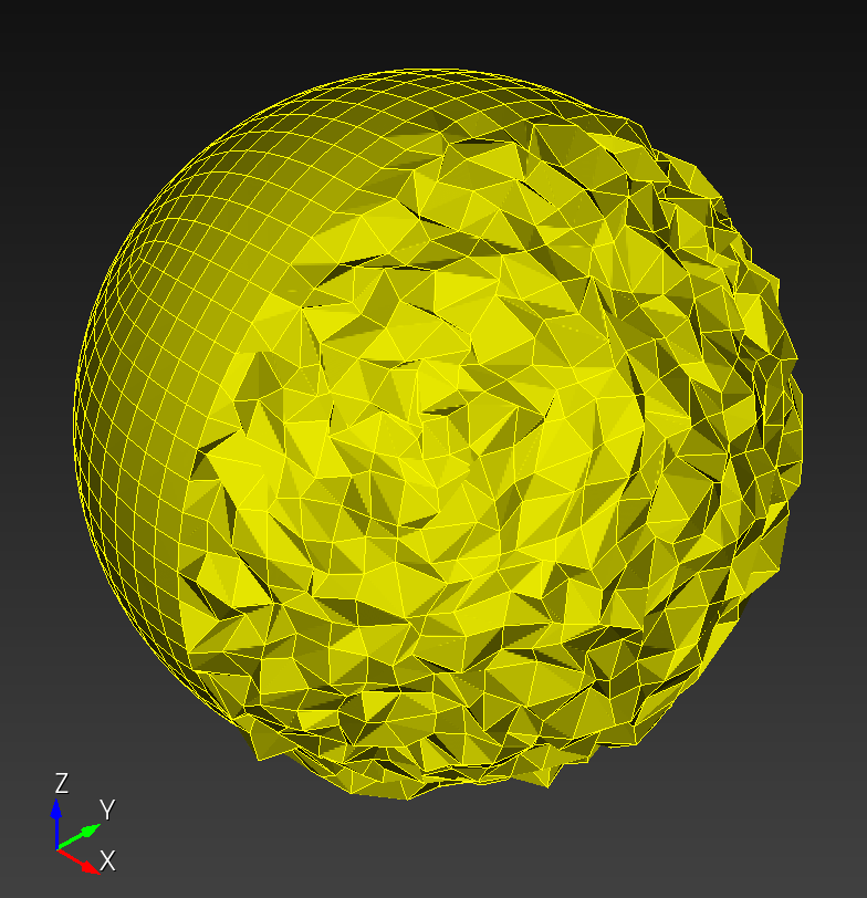 | 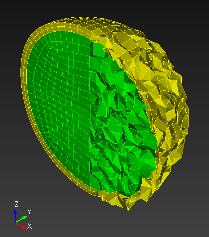 | 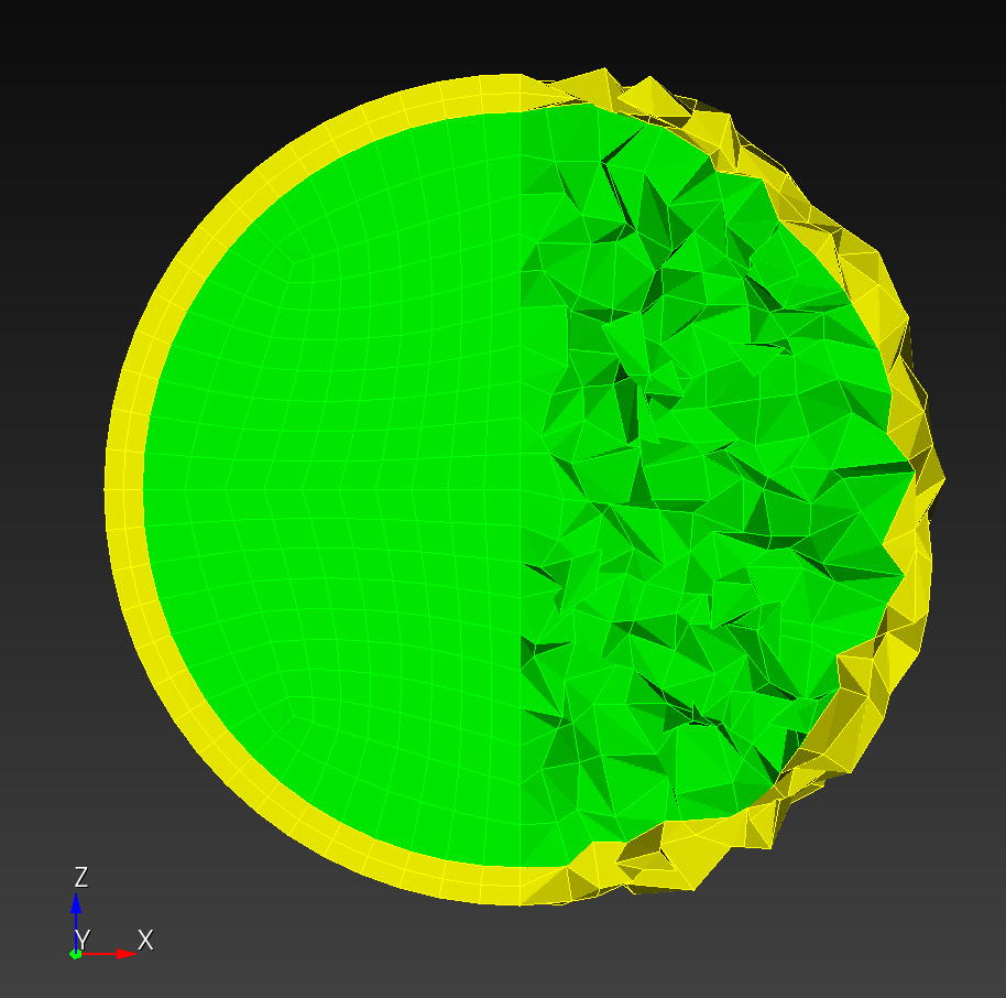 |
Figure 4.10-1: (Top row) sphere original configuration. (Bottom row) noised sphere configuration, with normal random nodal displacement of the coordinates where .
Taubin example
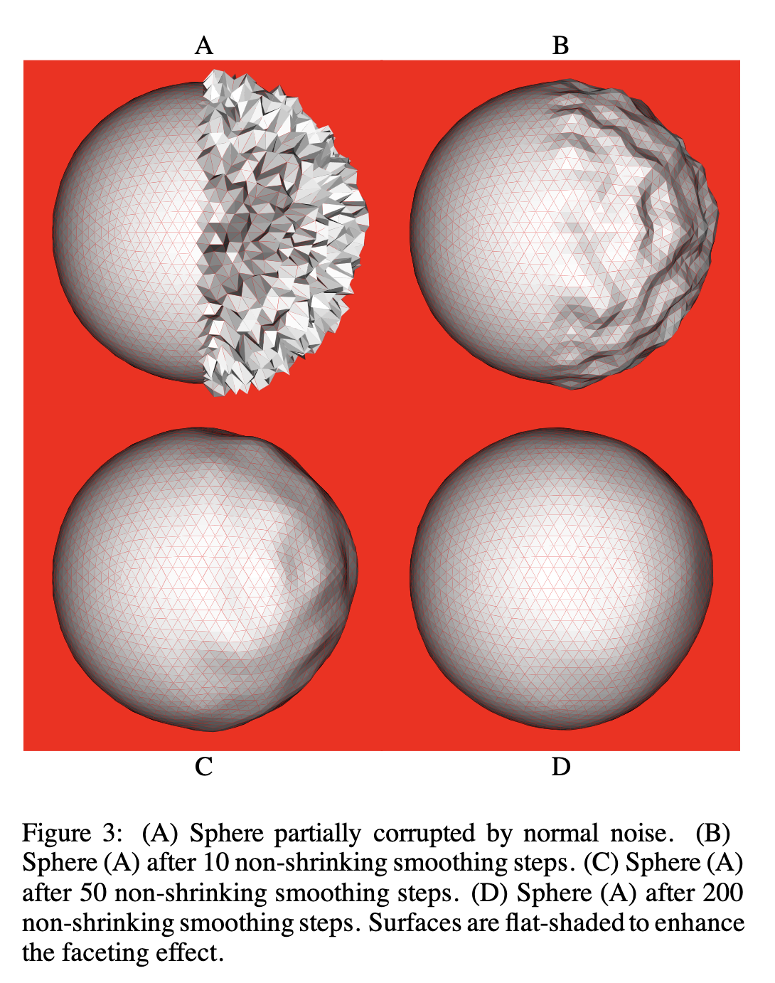
Figure 4.10-2: Excerpt from Taubin1, Figure 3, showing a surface mesh original configuration, and after 10, 50, and 200 steps.
automesh
We compare our volumetric results to the surface mesh presented by Taubin.1 A step is either a "shrinking step" (deflating, smoothing step) or an "un-shrinking step" (reinflating step).
The smoothing parameters used were the autotwin defaults,2 the same as used in Taubin's Figure 3 example.
The 10-iteration smooth command
automesh smooth -i sphere_res_1cm_noised.inp -o s10.exo -n 10
The 50-iteration smooth command
automesh smooth -i sphere_res_1cm_noised.inp -o s50.exo -n 50
The 200-iteration smooth command
automesh smooth -i sphere_res_1cm_noised.inp -o s200.exo -n 200
| front | iso | xz midplane |
|---|---|---|
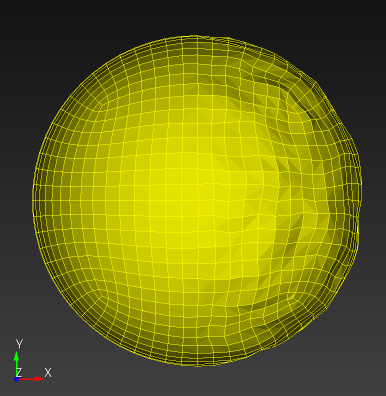 | 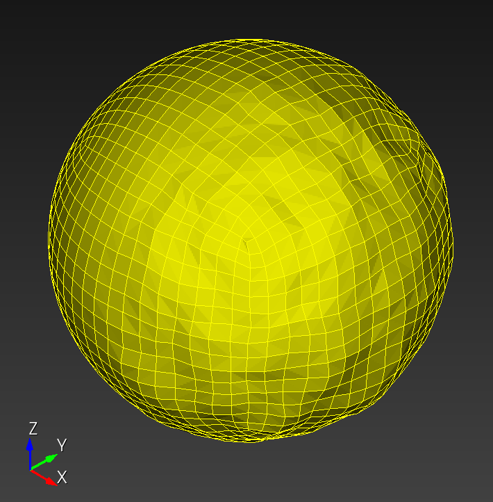 | 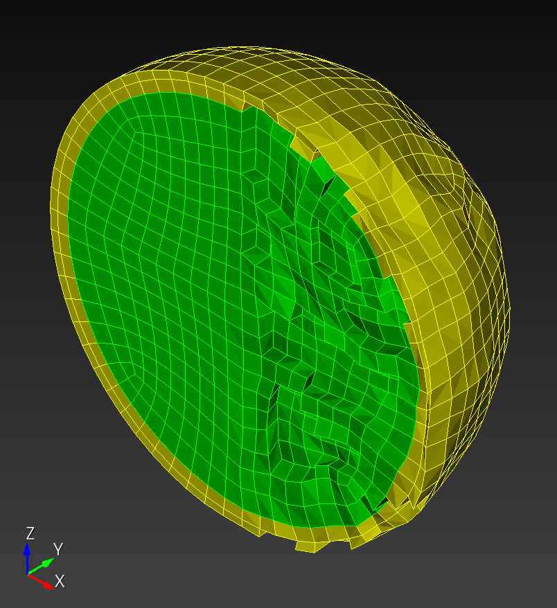 |
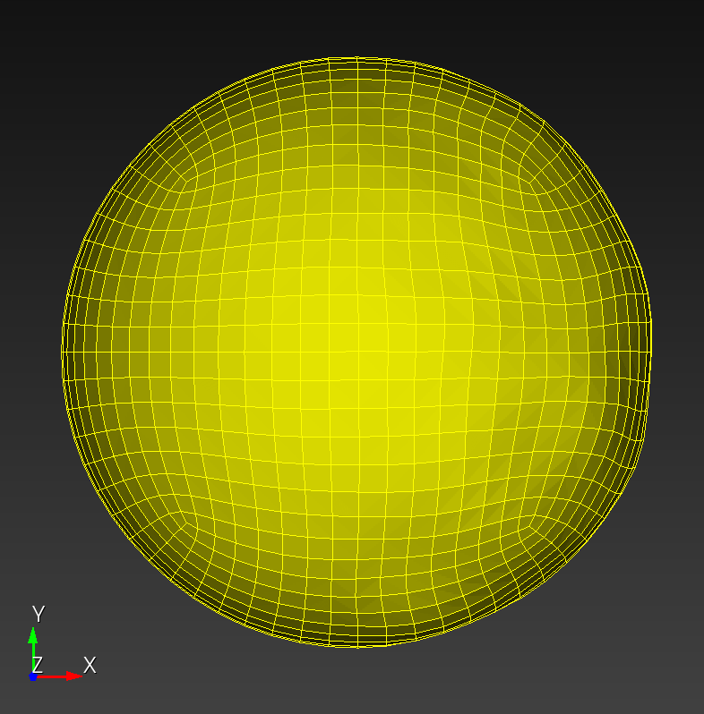 | 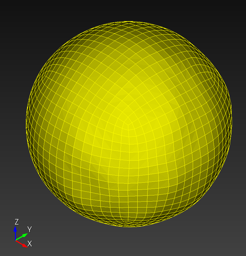 | 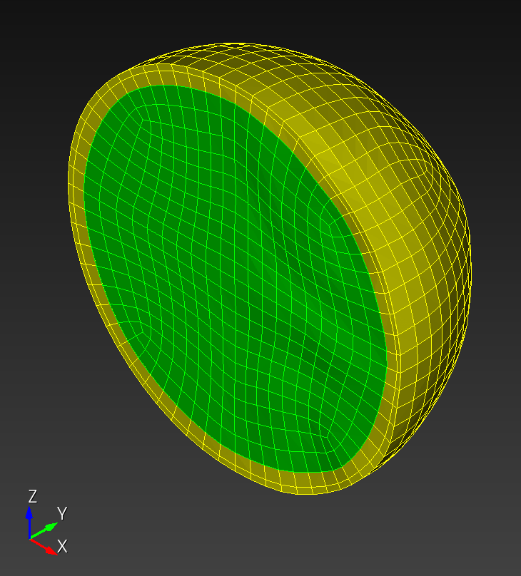 |
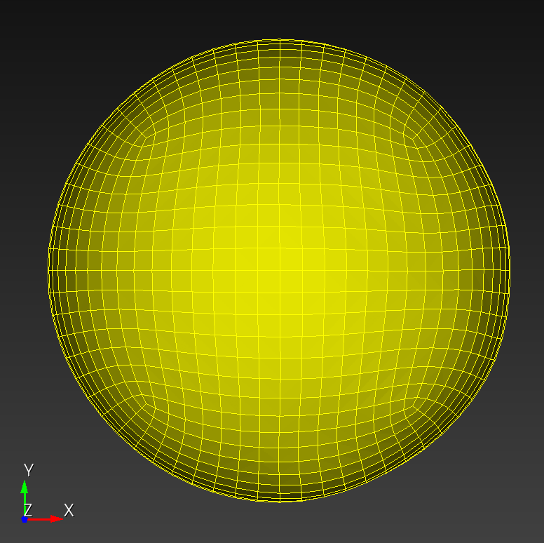 | 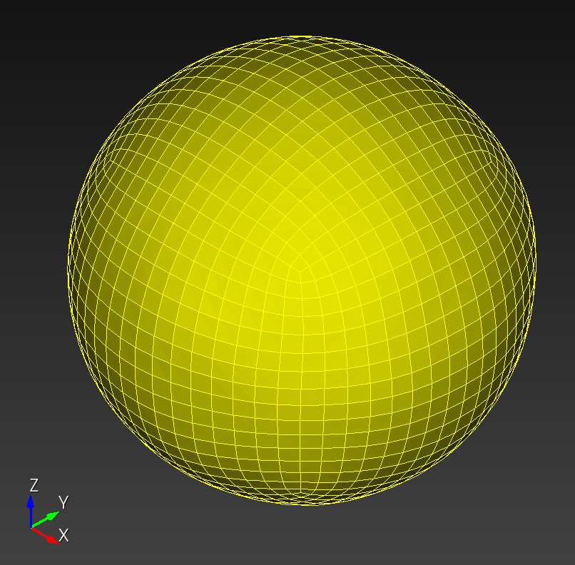 | 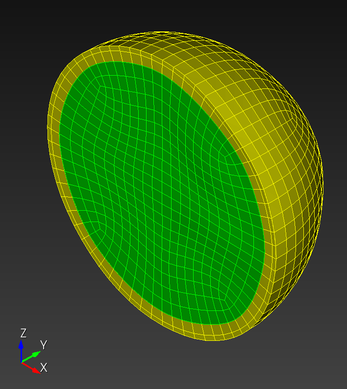 |
Figure 4.10-3: Smoothing results after 10 (top row), 50 (middle row), and 200 (bottom row) iterations.
The results demonstrate that our implementation of Taubin smoothing on volumetric meshes composed of hexahedral elements performs well. All smoothing operations completed within 7.5 ms. Unlike Laplace smoothing, which drastically reduces volume (e.g., -16% in 10 iterations), Taubin smoothing preserves volumes (e.g., +1% in 200 iterations). Thus, the noise in the hemisphere was effectively removed, with very small volumetric change. The hemisphere did not degrade from its original configuration.
Source
sphere.jou
sphere.jou
# Cubit 16.14 on macOS
# automesh/book/examples/smoothing/sphere.jou

reset

# ----------------
# INPUT PARAMETERS
# ----------------

# centimeters
# {INNER_RADIUS = 10.0} # cm
# {OUTER_RADIUS = 11.0} # cm
#
# {ELEMENT_SIZE = 1.0} # cm
#
# {UNITS = "cm"}

# {savefolder = "/Users/chovey/autotwin/basis/data/cubit/"}
# {savefolder = "/Users/chovey/autotwin/basis/scratch/"}
# {savefolder = "/Users/chovey/autotwin/automesh/book/examples/smoothing/"}

# {basename = "sphere_res_"}

# {str_exodus = savefolder//basename//tostring(ELEMENT_SIZE)//UNITS//".e"}
# {str_exodus = savefolder//basename//tostring(ELEMENT_SIZE)//UNITS//".g"}
# example:
# /Users/chovey/autotwin/basis/data/cubit/spheres_e_len_0.01m.e
# /Users/chovey/autotwin/basis/data/cubit/spheres_e_len_0.01m.g
# /Users/chovey/autotwin/basis/scratch/smooth_1cm.g

# {str_abaqus = savefolder//basename//tostring(ELEMENT_SIZE)//UNITS//".inp"}
# example:
# /Users/chovey/autotwin/basis/data/cubit/spheres_e_len_0.01m.inp
# /Users/chovey/autotwin/basis/scratch/smooth_1cm.inp

# {str_export_exodus = 'export mesh   "'//str_exodus// '" overwrite '}
# example:
# export mesh   "/Users/chovey/autotwin/basis/data/cubit/spheres_e_len_0.01m.e" overwrite
# export mesh   "/Users/chovey/autotwin/basis/data/cubit/spheres_e_len_0.01m.g" overwrite
# export mesh   "/Users/chovey/autotwin/basis/scratch/smooth_1cm.g" overwrite

# {str_export_abaqus = 'export abaqus "'//str_abaqus// '" overwrite everything'}
# example:
# export abaqus "/Users/chovey/autotwin/basis/data/cubit/spheres_e_len_0.01m.inp" overwrite everything
# export abaqus "/Users/chovey/autotwin/basis/scratch/smooth_1cm.inp" overwrite everything

#   From Sokolow, 2024-03-04-1725:
#   // in aprepro is string concatenation
#   I separated the folder from the file name just for readability.
#   The definition of “st” is to setup the folder+filename
#   The definition of “s2” is to prevent cubit/aprepro from getting confused with nested strings by using single quotes surrounding a solitary double quote.
#   The last line “rescan” actually tells cubit to process the whole string as a command.
#   The save folder definition I would put at the top of the journal file.

# -------------------
# DERIVED CALCUATIONS
# -------------------

# {OUTER_INTERVAL = max(2, ceil((OUTER_RADIUS - INNER_RADIUS)/ELEMENT_SIZE))}
# {ELEMENT_TOLERANCE = ELEMENT_SIZE/10000}
# {SELECTION_RADIUS = INNER_RADIUS/2.0}

create sphere radius {OUTER_RADIUS}
create sphere radius {INNER_RADIUS}
subtract volume 2 from volume 1 # creates new volume 3

create sphere radius {INNER_RADIUS} # creates new volume 4

section vol all yplane
section vol all zplane
section vol all xplane

imprint vol all
merge vol all

vol 4 rename "inner_vol"
vol 3 rename "outer_vol"
vol all size {ELEMENT_SIZE}
volume with name "inner_vol" scheme tetprimitive

# highlight curve with x_coord < 1.0 and with y_coord < 1.0 and with z_coord < 1.0

curve with x_coord < {SELECTION_RADIUS} and with y_coord < {SELECTION_RADIUS} and with z_coord < {SELECTION_RADIUS} interval {ceil(INNER_RADIUS/ELEMENT_SIZE)}
curve with x_coord < {SELECTION_RADIUS} and with y_coord < {SELECTION_RADIUS} and with z_coord < {SELECTION_RADIUS} scheme equal
mesh curve with x_coord < {SELECTION_RADIUS} and with y_coord < {SELECTION_RADIUS} and with z_coord < {SELECTION_RADIUS}

mesh volume with name "inner_vol"


curve 4 16 18 interval {OUTER_INTERVAL}
curve 4 16 18 scheme equal
mesh curve 4 16 18


volume with name "outer_vol" redistribute nodes off
# surface 19 is at the inner_vol radius
# surface 21 is at the outer_vol radius
volume with name "outer_vol" scheme sweep source surface 19    target surface 21    sweep transform least squares
volume with name "outer_vol"  autosmooth target on  fixed imprints off  smart smooth off
mesh volume with name "outer_vol"

Volume all copy reflect x

imprint vol all
merge vol all

Volume all copy reflect y

imprint vol all
merge vol all

Volume all copy reflect z

imprint vol all
merge vol all

block 1 volume with name "inner_vol*"
block 2 volume with name "outer_vol*"


# quality volume all shape global draw mesh

# export mesh "/Users/chovey/autotwin/basis/data/cubit/unmerged" + {ELEMENT_SIZE}.e  overwrite
# export mesh "/Users/chovey/autotwin/basis/data/cubit/unmerged.e"  overwrite
# export mesh "/Users/chovey/autotwin/basis/scratch/unmerged.e"  overwrite
export mesh "/Users/chovey/autotwin/automesh/book/examples/smoothing/sphere_temp_unmerged.g" overwrite

reset

# import mesh geometry "/Users/chovey/autotwin/basis/data/cubit/unmerged.e" feature_angle 135.00  merge  merge_nodes {ELEMENT_SIZE/100}
# import mesh geometry "/Users/chovey/autotwin/basis/data/cubit/unmerged.e" feature_angle 135.00  merge  merge_nodes {ELEMENT_TOLERANCE}
# import mesh geometry "/Users/chovey/autotwin/basis/scratch/unmerged.e" feature_angle 135.00  merge  merge_nodes {ELEMENT_TOLERANCE}
import mesh geometry "/Users/chovey/autotwin/automesh/book/examples/smoothing/sphere_temp_unmerged.g" merge  merge_nodes {ELEMENT_TOLERANCE}

sideset 1 add surface 1
sideset 2 add surface 2

# export mesh "/Users/chovey/autotwin/basis/scratch/smooth_1cm.g"  overwrite
# export abaqus "/Users/chovey/autotwin/basis/scratch/smooth_1cm.inp" overwrite everything
# inner_vol = block 1: 7,168 elements
# outer_vol = block 2: 3,072 elements
# total: 10,240 elements

{rescan(str_export_exodus)}
{rescan(str_export_abaqus)}

# view iso
# graphics clip on plane xplane location 0 0 0 direction 0 0 1
graphics scale off
graphics scale on

graphics clip off
view iso
graphics clip on plane location 0 0 0 direction 0 1 0
view up 0 0 1
view from 100 -100 100

graphics clip manipulation off

view bottom
noise_augmentation.py
noise_augmentation.py
r"""This module, noise_augmentation.py, adds noise to a finite element mesh
in the .inp format.

Example:
--------
source ~/autotwin/automesh/.venv/bin/activate
cd ~/autotwin/automesh/book/examples/smoothing
python noise_augmentation.py
"""

from pathlib import Path
from typing import Final
import random


FILE_INPUT: Final[Path] = Path(__file__).parent.joinpath("sphere_res_1cm.inp")
FILE_OUTPUT: Final[Path] = Path(__file__).parent.joinpath("sphere_res_1cm_noised.inp")
SEED_VALUE: Final[int] = 42  # set a seed value for reproducibility
random.seed(SEED_VALUE)
# AMP: Final[float] = 0.0  # the amplitude of the noise, debug
AMP: Final[float] = 0.5  # the amplitude of the noise


def has_e_plus_minus(string_in: str) -> bool:
    """Utility function, if the input string has the format
    "E+", "e+", "E-", or "E-", then return True, otherwise False.
    """
    return (
        "E+" in string_in or "e+" in string_in or "E-" in string_in or "e-" in string_in
    )


def has_four_entries(string_in: str) -> bool:
    """Utility function that evaluates a string.  If the input has four
    entries, which is the format of the nodal coordinates, then return
    True, otherwise, return False."""
    return len(string_in.split(",")) == 4


with (
    open(FILE_INPUT, "r", encoding="utf-8") as fin,
    open(FILE_OUTPUT, "w", encoding="utf-8") as fout,
):
    for line in fin:
        # print(line)  # debugging
        if has_four_entries(line):
            # This might be a coordinate, investigate further.
            items = line.split(",")
            node, px, py, pz = tuple(i.strip() for i in items)

            # if all coordinates have the E+/e+ or E-/e- notation
            if all(has_e_plus_minus(k) for k in [px, py, pz]):
                # we noise only coordinates on the positive x half-space
                if float(px) > 0.0:
                    # Pick three random number between -1 and 1
                    rx = random.uniform(-1, 1)
                    ry = random.uniform(-1, 1)
                    rz = random.uniform(-1, 1)
                    # create the noise values
                    nx = AMP * rx
                    ny = AMP * ry
                    nz = AMP * rz
                    # create noisy values
                    qx = float(px) + nx
                    qy = float(py) + ny
                    qz = float(pz) + nz
                    formatted_line = (
                        f"{node:>8}, {qx:>15.6e}, {qy:>15.6e}, {qz:>15.6e}\n"
                    )
                    line = formatted_line  # overwrite with new noised line

        fout.write(line)

print(f"Wrote {FILE_OUTPUT}")
print("Done.")
References
-
Taubin G. A signal processing approach to fair surface design. In Proceedings of the 22nd annual conference on Computer graphics and interactive techniques 1995 Sep 15 (pp. 351-358). paper ↩ ↩2
-
autotwindefault Taubin parameters: , . ↩
Python Visualization
Following are files to support the Python visualization.
smoothing_types.py
smoothing_types.py
r"""This module, smoothing_types.py, defines types used for smoothing
hexahedral meshes.
"""

from enum import Enum
from typing import NamedTuple


class Vertex(NamedTuple):
    """A general 3D vertex with x, y, and z coordinates."""

    x: float
    y: float
    z: float


class Hierarchy(Enum):
    """All nodes must be categorized as belonging to one, and only one,
    of the following hierarchical categories.
    """

    INTERIOR = 0
    BOUNDARY = 1
    PRESCRIBED = 2


Vertices = tuple[Vertex, ...]
Hex = tuple[int, int, int, int, int, int, int, int]  # only hex elements
Hexes = tuple[Hex, ...]
Neighbor = tuple[int, ...]
Neighbors = tuple[Neighbor, ...]
NodeHierarchy = tuple[Hierarchy, ...]
PrescribedNodes = tuple[tuple[int, Vertex], ...] | None


class SmoothingAlgorithm(Enum):
    """The type of smoothing algorithm."""

    LAPLACE = "Laplace"
    TAUBIN = "Taubin"


class SmoothingExample(NamedTuple):
    """The prototype smoothing example."""

    vertices: Vertices
    elements: Hexes
    nelx: int
    nely: int
    nelz: int
    # neighbors: Neighbors
    node_hierarchy: NodeHierarchy
    prescribed_nodes: PrescribedNodes
    scale_lambda: float
    scale_mu: float
    num_iters: int
    algorithm: SmoothingAlgorithm
    file_stem: str
smoothing_test.py
smoothing_test.py
r"""This module, smoothing_test.py, tests the smoothing modules.

Example:
--------
source ~/autotwin/automesh/.venv/bin/activate
cd ~/autotwin/automesh/book/examples/smoothing
python -m pytest smoothing_test.py

Reference:
----------
DoubleX unit test
https://autotwin.github.io/automesh/examples/unit_tests/index.html#double-x
"""

from typing import Final

# import sandbox.smoothing as sm
# import sandbox.smoothing_types as ty
import smoothing as sm
import smoothing_examples as examples
import smoothing_types as ty

# Type alias for functional style methods
# https://docs.python.org/3/library/typing.html#type-aliases
Hexes = ty.Hexes
Hierarchy = ty.Hierarchy
Neighbors = ty.Neighbors
NodeHierarchy = ty.NodeHierarchy
Vertex = ty.Vertex
Vertices = ty.Vertices
SmoothingAlgorithm = ty.SmoothingAlgorithm


def test_average_position():
    """Unit test for average_position"""
    v1 = Vertex(x=1.0, y=2.0, z=3.0)
    v2 = Vertex(x=4.0, y=5.0, z=6.0)
    v3 = Vertex(x=7.0, y=8.0, z=9.0)

    v_ave = sm.average_position((v1, v2, v3))
    assert v_ave.x == 4.0
    assert v_ave.y == 5.0
    assert v_ave.z == 6.0

    # docstring example
    v1, v2 = Vertex(1, 2, 3), Vertex(4, 5, 6)
    assert sm.average_position((v1, v2)) == Vertex(2.5, 3.5, 4.5)


def test_add():
    """Unit test for the addition of Vertex v1 and Vertex v2."""
    v1 = Vertex(x=1.0, y=2.0, z=3.0)
    v2 = Vertex(x=4.0, y=7.0, z=1.0)
    vv = sm.add(v1=v1, v2=v2)
    assert vv.x == 5.0
    assert vv.y == 9.0
    assert vv.z == 4.0

    # docstring example
    v1, v2 = Vertex(1, 2, 3), Vertex(4, 5, 6)
    assert sm.add(v1, v2) == Vertex(5, 7, 9)


def test_subtract():
    """Unit test for the subtraction of Vertex v2 from Vertex v1."""
    v1 = Vertex(x=1.0, y=2.0, z=3.0)
    v2 = Vertex(x=4.0, y=7.0, z=1.0)
    vv = sm.subtract(v1=v1, v2=v2)
    assert vv.x == -3.0
    assert vv.y == -5.0
    assert vv.z == 2.0

    # docstring example
    v1, v2 = Vertex(8, 5, 2), Vertex(1, 2, 3)
    assert sm.subtract(v1, v2) == Vertex(7, 3, -1)


def test_scale():
    """Unit test for the scale function."""
    v1 = Vertex(x=1.0, y=2.0, z=3.0)
    ss = 10.0
    result = sm.scale(vertex=v1, scale_factor=ss)
    assert result.x == 10.0
    assert result.y == 20.0
    assert result.z == 30.0

    # docstring example
    v = Vertex(1, 2, 3)
    scale_factor = 2
    assert sm.scale(v, scale_factor) == Vertex(2, 4, 6)


def test_xyz():
    """Unit test to assure the (x, y, z) coordinate tuple is returned
    correctly.
    """
    vv = Vertex(x=1.1, y=2.2, z=3.3)
    gold = (1.1, 2.2, 3.3)
    result = sm.xyz(vv)
    assert result == gold

    # docstring example
    v = Vertex(1, 2, 3)
    assert sm.xyz(v) == (1, 2, 3)


def test_smoothing_neighbors():
    """Given the Double X test problem with completely made up
    node hierarchy, assure that `smoothing_neighbors` returns
    the correct neighbors.
    """
    ex = examples.double_x
    # neighbors = ex.neighbors  # borrow the neighbor connections
    neighbors = sm.node_node_connectivity(ex.elements)

    node_hierarchy = (
        Hierarchy.INTERIOR,
        Hierarchy.BOUNDARY,
        Hierarchy.PRESCRIBED,
        Hierarchy.PRESCRIBED,
        Hierarchy.BOUNDARY,
        Hierarchy.INTERIOR,
        Hierarchy.INTERIOR,
        Hierarchy.BOUNDARY,
        Hierarchy.BOUNDARY,
        Hierarchy.INTERIOR,
        Hierarchy.INTERIOR,
        Hierarchy.INTERIOR,
    )

    result = sm.smoothing_neighbors(neighbors=neighbors, node_hierarchy=node_hierarchy)
    gold_smoothing_neighbors = (
        (2, 4, 7),
        (3, 5, 8),
        (),
        (),
        (2, 4),
        (3, 5, 12),
        (1, 8, 10),
        (2, 9),
        (3, 8),
        (4, 7, 11),
        (5, 8, 10, 12),
        (6, 9, 11),
    )

    assert result == gold_smoothing_neighbors

    # docstring example
    neighbors = ((2, 3), (1, 4), (1, 5), (2, 6), (3,), (4,))
    node_hierarchy = (
        Hierarchy.INTERIOR,
        Hierarchy.BOUNDARY,
        Hierarchy.PRESCRIBED,
        Hierarchy.BOUNDARY,
        Hierarchy.INTERIOR,
        Hierarchy.INTERIOR,
    )
    gold = ((2, 3), (4,), (), (2,), (3,), (4,))
    assert sm.smoothing_neighbors(neighbors, node_hierarchy) == gold


def test_laplace_hierarchical_bracket():
    """Unit test for Laplace smoothing with hierarchical control
    on the Bracket example."""
    bracket = examples.bracket

    node_hierarchy = bracket.node_hierarchy
    # neighbors = bracket.neighbors
    neighbors = sm.node_node_connectivity(bracket.elements)
    node_hierarchy = bracket.node_hierarchy

    # If a node is PRESCRIBED, then it has no smoothing neighbors
    smoothing_neighbors = sm.smoothing_neighbors(
        neighbors=neighbors, node_hierarchy=node_hierarchy
    )
    gold_smoothing_neighbors = (
        (),  # 1
        (),  # 2
        (),  # 3
        (),  # 4
        (),  # 5
        (),  # 6
        (2, 6, 8, 12, 28),  # 7
        (3, 7, 9, 13, 29),  # 8
        (4, 8, 10, 14, 30),  # 9
        (),  # 10
        (),  # 11
        (7, 11, 13, 17, 33),  # 12
        (8, 12, 14, 18, 34),  # 13
        (9, 13, 15, 35),  # 14
        (),  # 15
        (),  # 16
        (12, 16, 18, 20, 38),  # 17
        (13, 17, 21, 39),  # 18
        (),  # 19
        (),  # 20
        (),
        (),  # 22
        (),
        (),  # 24
        (),
        (),  # 26
        (),
        (7, 23, 27, 29, 33),  # 28
        (8, 24, 28, 30, 34),  # 29
        (9, 25, 29, 31, 35),  # 30
        (),  # 31
        (),  # 32
        (12, 28, 32, 34, 38),  # 33
        (13, 29, 33, 35, 39),  # 34
        (14, 30, 34, 36),  # 35
        (),  # 36
        (),  # 37
        (17, 33, 37, 39, 41),  # 38
        (18, 34, 38, 42),  # 39
        (),  # 40
        (),  # 41
        (),  # 42
    )

    assert smoothing_neighbors == gold_smoothing_neighbors

    # specific test with lambda = 0.3 and num_iters = 10
    scale_lambda_test = 0.3
    num_iters_test = 10

    result = sm.smooth(
        vv=bracket.vertices,
        hexes=bracket.elements,
        node_hierarchy=bracket.node_hierarchy,
        prescribed_nodes=bracket.prescribed_nodes,
        scale_lambda=scale_lambda_test,
        num_iters=num_iters_test,
        algorithm=bracket.algorithm,
    )

    gold_vertices_10_iter = (
        Vertex(x=0, y=0, z=0),
        Vertex(x=1, y=0, z=0),
        Vertex(x=2, y=0, z=0),
        Vertex(x=3, y=0, z=0),
        Vertex(x=4, y=0, z=0),
        Vertex(x=0, y=1, z=0),
        Vertex(x=0.9974824535030984, y=0.9974824535030984, z=0.24593434133370803),
        Vertex(x=1.9620726956646117, y=1.0109475009958278, z=0.2837944855813176),
        Vertex(x=2.848322987789396, y=1.1190213008349328, z=0.24898414051620496),
        Vertex(x=3.695518130045147, y=1.5307337294603591, z=0),
        Vertex(x=0, y=2, z=0),
        Vertex(x=1.0109475009958275, y=1.9620726956646117, z=0.2837944855813176),
        Vertex(x=1.9144176939366933, y=1.9144176939366933, z=0.3332231502067546),
        Vertex(x=2.5912759493290007, y=1.961874667390146, z=0.29909606343914835),
        Vertex(x=2.8284271247461903, y=2.82842712474619, z=0),
        Vertex(x=0, y=3, z=0),
        Vertex(x=1.119021300834933, y=2.848322987789396, z=0.24898414051620493),
        Vertex(x=1.9618746673901462, y=2.5912759493290007, z=0.29909606343914835),
        Vertex(x=0, y=4, z=0),
        Vertex(x=1.5307337294603593, y=3.695518130045147, z=0),
        Vertex(x=2.8284271247461903, y=2.82842712474619, z=0),
        Vertex(x=0, y=0, z=1),
        Vertex(x=1, y=0, z=1),
        Vertex(x=2, y=0, z=1),
        Vertex(x=3, y=0, z=1),
        Vertex(x=4, y=0, z=1),
        Vertex(x=0, y=1, z=1),
        Vertex(x=0.9974824535030984, y=0.9974824535030984, z=0.7540656586662919),
        Vertex(x=1.9620726956646117, y=1.0109475009958278, z=0.7162055144186824),
        Vertex(x=2.848322987789396, y=1.119021300834933, z=0.7510158594837951),
        Vertex(x=3.695518130045147, y=1.5307337294603591, z=1),
        Vertex(x=0, y=2, z=1),
        Vertex(x=1.0109475009958275, y=1.9620726956646117, z=0.7162055144186824),
        Vertex(x=1.9144176939366933, y=1.9144176939366933, z=0.6667768497932453),
        Vertex(x=2.591275949329001, y=1.9618746673901462, z=0.7009039365608517),
        Vertex(x=2.8284271247461903, y=2.82842712474619, z=1),
        Vertex(x=0, y=3, z=1),
        Vertex(x=1.1190213008349328, y=2.848322987789396, z=0.751015859483795),
        Vertex(x=1.9618746673901462, y=2.5912759493290007, z=0.7009039365608516),
        Vertex(x=0, y=4, z=1),
        Vertex(x=1.5307337294603593, y=3.695518130045147, z=1),
        Vertex(x=2.8284271247461903, y=2.82842712474619, z=1),
    )

    assert result == gold_vertices_10_iter


def test_laplace_smoothing_double_x():
    """Unit test for Laplace smoothing with all dofs as BOUNDARY
    on the Double X example."""
    vv: Vertices = (
        Vertex(0.0, 0.0, 0.0),
        Vertex(1.0, 0.0, 0.0),
        Vertex(2.0, 0.0, 0.0),
        Vertex(0.0, 1.0, 0.0),
        Vertex(1.0, 1.0, 0.0),
        Vertex(2.0, 1.0, 0.0),
        Vertex(0.0, 0.0, 1.0),
        Vertex(1.0, 0.0, 1.0),
        Vertex(2.0, 0.0, 1.0),
        Vertex(0.0, 1.0, 1.0),
        Vertex(1.0, 1.0, 1.0),
        Vertex(2.0, 1.0, 1.0),
    )

    hexes: Hexes = (
        (1, 2, 5, 4, 7, 8, 11, 10),
        (2, 3, 6, 5, 8, 9, 12, 11),
    )

    # nn: Neighbors = (
    #     (2, 4, 7),
    #     (1, 3, 5, 8),
    #     (2, 6, 9),
    #     (1, 5, 10),
    #     (2, 4, 6, 11),
    #     (3, 5, 12),
    #     (1, 8, 10),
    #     (2, 7, 9, 11),
    #     (3, 8, 12),
    #     (4, 7, 11),
    #     (5, 8, 10, 12),
    #     (6, 9, 11),
    # )

    nh: NodeHierarchy = (
        Hierarchy.BOUNDARY,
        Hierarchy.BOUNDARY,
        Hierarchy.BOUNDARY,
        Hierarchy.BOUNDARY,
        Hierarchy.BOUNDARY,
        Hierarchy.BOUNDARY,
        Hierarchy.BOUNDARY,
        Hierarchy.BOUNDARY,
        Hierarchy.BOUNDARY,
        Hierarchy.BOUNDARY,
        Hierarchy.BOUNDARY,
        Hierarchy.BOUNDARY,
    )

    scale_lambda: Final[float] = 0.3  # lambda for Laplace smoothing

    # iteration 1
    num_iters = 1  # single iteration of smoothing

    algo = SmoothingAlgorithm.LAPLACE

    aa = sm.smooth(
        vv=vv,
        hexes=hexes,
        node_hierarchy=nh,
        prescribed_nodes=None,
        scale_lambda=scale_lambda,
        num_iters=num_iters,
        algorithm=algo,
    )
    cc: Final[float] = scale_lambda / 3.0  # delta corner
    ee: Final[float] = scale_lambda / 4.0  # delta edge
    # define the gold standard fiducial
    gold = (
        Vertex(x=cc, y=cc, z=cc),  # node 1, corner
        Vertex(x=1.0, y=ee, z=ee),  # node 2, edge
        Vertex(x=2.0 - cc, y=cc, z=cc),  # node 3, corner
        #
        Vertex(x=cc, y=1.0 - cc, z=cc),  # node 4, corner
        Vertex(x=1.0, y=1.0 - ee, z=ee),  # node 5, edge
        Vertex(x=2.0 - cc, y=1.0 - cc, z=cc),  # node 6, corner
        #
        Vertex(x=cc, y=cc, z=1 - cc),  # node 7, corner
        Vertex(x=1.0, y=ee, z=1 - ee),  # node 8, edge
        Vertex(x=2.0 - cc, y=cc, z=1 - cc),  # node 9, corner
        #
        Vertex(x=cc, y=1.0 - cc, z=1 - cc),  # node 10, corner
        Vertex(x=1.0, y=1.0 - ee, z=1 - ee),  # node 11, edge
        Vertex(x=2.0 - cc, y=1.0 - cc, z=1 - cc),  # node 12, corner
    )
    assert aa == gold

    # iteration 2
    num_iters = 2  # overwrite, double iteration of smoothing

    aa2 = sm.smooth(
        vv=vv,
        hexes=hexes,
        node_hierarchy=nh,
        prescribed_nodes=None,
        scale_lambda=scale_lambda,
        num_iters=num_iters,
        algorithm=algo,
    )
    # define the gold standard fiducial
    gold2 = (
        (0.19, 0.1775, 0.1775),
        (1.0, 0.1425, 0.1425),
        (1.8099999999999998, 0.1775, 0.1775),
        (0.19, 0.8225, 0.1775),
        (1.0, 0.8575, 0.1425),
        (1.8099999999999998, 0.8225, 0.1775),
        (0.19, 0.1775, 0.8225),
        (1.0, 0.1425, 0.8575),
        (1.8099999999999998, 0.1775, 0.8225),
        (0.19, 0.8225, 0.8225),
        (1.0, 0.8575, 0.8575),
        (1.8099999999999998, 0.8225, 0.8225),
    )
    assert aa2 == gold2


def test_pair_ordered():
    """Unit test for pair ordered."""

    # small toy example
    given = ((3, 1), (2, 1))
    found = sm.pair_ordered(given)
    gold = ((1, 2), (1, 3))
    assert found == gold

    # example from 12 edges of a hex element
    given = (
        (1, 2),
        (2, 5),
        (4, 1),
        (5, 4),
        (7, 8),
        (8, 11),
        (11, 10),
        (10, 7),
        (1, 7),
        (2, 8),
        (5, 11),
        (4, 10),
    )  # overwrite
    gold = (
        (1, 2),
        (1, 4),
        (1, 7),
        (2, 5),
        (2, 8),
        (4, 5),
        (4, 10),
        (5, 11),
        (7, 8),
        (7, 10),
        (8, 11),
        (10, 11),
    )  # overwrite
    found = sm.pair_ordered(given)  # overwrite
    assert found == gold

    # docstring example
    pairs = ((3, 1), (2, 4), (5, 0))
    assert sm.pair_ordered(pairs) == ((0, 5), (1, 3), (2, 4))


def test_edge_pairs():
    """Units test to assure edge pairs are computed correctly."""
    elements = (
        (1, 2, 5, 4, 7, 8, 11, 10),
        (2, 3, 6, 5, 8, 9, 12, 11),
    )
    found = sm.edge_pairs(hexes=elements)
    gold = (
        (1, 2),
        (1, 4),
        (1, 7),
        (2, 3),
        (2, 5),
        (2, 8),
        (3, 6),
        (3, 9),
        (4, 5),
        (4, 10),
        (5, 6),
        (5, 11),
        (6, 12),
        (7, 8),
        (7, 10),
        (8, 9),
        (8, 11),
        (9, 12),
        (10, 11),
        (11, 12),
    )
    assert found == gold


def test_node_node_connectivity():
    """Tests that the node_node_connectivity function is properly
    implemented.
    """

    # from the Double X unit test

    hexes = (
        (1, 2, 5, 4, 7, 8, 11, 10),
        (2, 3, 6, 5, 8, 9, 12, 11),
    )

    gold_neighbors = (
        (2, 4, 7),
        (1, 3, 5, 8),
        (2, 6, 9),
        (1, 5, 10),
        (2, 4, 6, 11),
        (3, 5, 12),
        (1, 8, 10),
        (2, 7, 9, 11),
        (3, 8, 12),
        (4, 7, 11),
        (5, 8, 10, 12),
        (6, 9, 11),
    )

    result = sm.node_node_connectivity(hexes)

    assert gold_neighbors == result

    # now with node number modifications to assure the
    # algorithm does not assume sequential node numbers:
    # 2 -> 22
    # 5 -> 55
    # 8 -> 88
    # 11 -> 111
    hexes_2 = (
        (1, 22, 55, 4, 7, 88, 111, 10),
        (22, 3, 6, 55, 88, 9, 12, 111),
    )

    gold_neighbors_2 = (
        (4, 7, 22),  # 1
        (6, 9, 22),  # 3
        (1, 10, 55),  # 4
        (3, 12, 55),  # 6
        (1, 10, 88),  # 7
        (3, 12, 88),  # 9
        (4, 7, 111),  # 10
        (6, 9, 111),  # 12
        (1, 3, 55, 88),  # 2 -> 22
        (4, 6, 22, 111),  # 5 -> 55
        (7, 9, 22, 111),  # 8 -> 88
        (10, 12, 55, 88),  # 11 -> 111
    )

    result_2 = sm.node_node_connectivity(hexes_2)

    assert gold_neighbors_2 == result_2

    # example from the L-bracket example
    hexes_bracket = (
        (1, 2, 7, 6, 22, 23, 28, 27),
        (2, 3, 8, 7, 23, 24, 29, 28),
        (3, 4, 9, 8, 24, 25, 30, 29),
        (4, 5, 10, 9, 25, 26, 31, 30),
        (6, 7, 12, 11, 27, 28, 33, 32),
        (7, 8, 13, 12, 28, 29, 34, 33),
        (8, 9, 14, 13, 29, 30, 35, 34),
        (9, 10, 15, 14, 30, 31, 36, 35),
        (11, 12, 17, 16, 32, 33, 38, 37),
        (12, 13, 18, 17, 33, 34, 39, 38),
        (16, 17, 20, 19, 37, 38, 41, 40),
        (17, 18, 21, 20, 38, 39, 42, 41),
    )

    gold_neighbors_bracket = (
        (2, 6, 22),
        (1, 3, 7, 23),
        (2, 4, 8, 24),
        (3, 5, 9, 25),
        (4, 10, 26),
        #
        (1, 7, 11, 27),
        (2, 6, 8, 12, 28),
        (3, 7, 9, 13, 29),
        (4, 8, 10, 14, 30),
        (5, 9, 15, 31),
        #
        (6, 12, 16, 32),
        (7, 11, 13, 17, 33),
        (8, 12, 14, 18, 34),
        (9, 13, 15, 35),
        (10, 14, 36),
        #
        (11, 17, 19, 37),
        (12, 16, 18, 20, 38),
        (13, 17, 21, 39),
        #
        (16, 20, 40),
        (17, 19, 21, 41),
        (18, 20, 42),
        # top layer
        (1, 23, 27),
        (2, 22, 24, 28),
        (3, 23, 25, 29),
        (4, 24, 26, 30),
        (5, 25, 31),
        #
        (6, 22, 28, 32),
        (7, 23, 27, 29, 33),
        (8, 24, 28, 30, 34),
        (9, 25, 29, 31, 35),
        (10, 26, 30, 36),
        #
        (11, 27, 33, 37),
        (12, 28, 32, 34, 38),
        (13, 29, 33, 35, 39),
        (14, 30, 34, 36),
        (15, 31, 35),
        #
        (16, 32, 38, 40),
        (17, 33, 37, 39, 41),
        (18, 34, 38, 42),
        #
        (19, 37, 41),
        (20, 38, 40, 42),
        (21, 39, 41),
    )

    result_bracket = sm.node_node_connectivity(hexes_bracket)

    assert gold_neighbors_bracket == result_bracket
smoothing.py
smoothing.py
r"""This module, smoothing.py, contains the core computations for
smoothing algorithms.
"""

# import sandbox.smoothing_types as ty
import smoothing_types as ty


# Type alias for functional style methods
# https://docs.python.org/3/library/typing.html#type-aliases
Hexes = ty.Hexes
Hierarchy = ty.Hierarchy
Neighbors = ty.Neighbors
NodeHierarchy = ty.NodeHierarchy
PrescribedNodes = ty.PrescribedNodes
Vertex = ty.Vertex
Vertices = ty.Vertices
SmoothingAlgorithm = ty.SmoothingAlgorithm


def average_position(vertices: Vertices) -> Vertex:
    """Calculate the average position of a list of vertices.

    This function computes the average coordinates (x, y, z) of a given
    list of Vertex objects. It raises an assertion error if the input
    list is empty.

    Parameters:
    vertices (Vertices): A list or collection of Vertex objects, where
                         each Vertex has x, y, and z attributes
                         representing its coordinates in 3D space.

    Returns:
    Vertex: A new Vertex object representing the average position of the
            input vertices, with x, y, and z attributes set to the
            average coordinates.

    Raises:
    AssertionError: If the number of vertices is zero, indicating that
                    the input list must contain at least one vertex.

    Example:
    >>> v1 = Vertex(1, 2, 3)
    >>> v2 = Vertex(4, 5, 6)
    >>> average_position([v1, v2])
    Vertex(x=2.5, y=3.5, z=4.5)
    """

    n_vertices = len(vertices)
    assert n_vertices > 0, "Error: number of vertices must be positive."
    xs = [v.x for v in vertices]
    ys = [v.y for v in vertices]
    zs = [v.z for v in vertices]
    x_ave = sum(xs) / n_vertices
    y_ave = sum(ys) / n_vertices
    z_ave = sum(zs) / n_vertices

    return Vertex(x=x_ave, y=y_ave, z=z_ave)


def add(v1: Vertex, v2: Vertex) -> Vertex:
    """
    Add two Vertex objects component-wise.

    This function takes two Vertex objects and returns a new Vertex
    object that represents the component-wise addition of the two
    input vertices.

    Parameters:
    v1 (Vertex): The first Vertex object to be added.
    v2 (Vertex): The second Vertex object to be added.

    Returns:
    Vertex: A new Vertex object representing the result of the addition,
            with x, y, and z attributes set to the sum of the corresponding
            attributes of v1 and v2.

    Example:
    >>> v1 = Vertex(1, 2, 3)
    >>> v2 = Vertex(4, 5, 6)
    >>> add(v1, v2)
    Vertex(x=5, y=7, z=9)
    """
    dx = v1.x + v2.x
    dy = v1.y + v2.y
    dz = v1.z + v2.z
    return Vertex(x=dx, y=dy, z=dz)


def subtract(v1: Vertex, v2: Vertex) -> Vertex:
    """
    Subtract one Vertex object from another component-wise.

    This function takes two Vertex objects and returns a new Vertex
    object that represents the component-wise subtraction of the second
    vertex from the first.

    Parameters:
    v1 (Vertex): The Vertex object from which v2 will be subtracted.
    v2 (Vertex): The Vertex object to be subtracted from v1.

    Returns:
    Vertex: A new Vertex object representing the result of the subtraction,
            (v1 - v2), with x, y, and z attributes set to the difference
            of the corresponding attributes of v1 and v2.

    Example:
    >>> v1 = Vertex(8, 5, 2)
    >>> v2 = Vertex(1, 2, 3)
    >>> subtract(v1, v2)
    Vertex(x=7, y=3, z=-1)
    """
    dx = v1.x - v2.x
    dy = v1.y - v2.y
    dz = v1.z - v2.z
    return Vertex(x=dx, y=dy, z=dz)


def scale(vertex: Vertex, scale_factor: float) -> Vertex:
    """
    Scale a Vertex object by a given scale factor.

    This function takes a Vertex object and a scale factor, and returns
    a new Vertex object that represents the original vertex scaled by
    the specified factor.

    Parameters:
    vertex (Vertex): The Vertex object to be scaled.
    scale_factor (float): The factor by which to scale the vertex.
                          This can be any real number, including
                          positive, negative, or zero.

    Returns:
    Vertex: A new Vertex object representing the scaled vertex, with
            x, y, and z attributes set to the original coordinates
            multiplied by the scale factor.

    Example:
    >>> v = Vertex(1, 2, 3)
    >>> scale_factor = 2
    >>> scale(v, scale_factor)
    Vertex(x=2, y=4, z=6)
    """
    x = scale_factor * vertex.x
    y = scale_factor * vertex.y
    z = scale_factor * vertex.z
    return Vertex(x=x, y=y, z=z)


def xyz(v1: Vertex) -> tuple[float, float, float]:
    """
    Extract the coordinates of a Vertex object.

    This function takes a Vertex object and returns its coordinates
    as a tuple in the form (x, y, z).

    Parameters:
    v1 (Vertex): The Vertex object from which to extract the coordinates.

    Returns:
    tuple[float, float, float]: A tuple containing the x, y, and z
                                 coordinates of the vertex.

    Example:
    >>> v = Vertex(1, 2, 3)
    >>> xyz(v)
    (1, 2, 3)
    """
    aa, bb, cc = v1.x, v1.y, v1.z
    return (aa, bb, cc)


def smoothing_neighbors(neighbors: Neighbors, node_hierarchy: NodeHierarchy):
    """
    Determine the smoothing neighbors for each node based on its
    hierarchy level.

    This function takes an original neighbors structure, which is defined
    by the connectivity of a mesh, and a node hierarchy. It returns a
    subset of the original neighbors that are used for smoothing, based
    on the hierarchy levels of the nodes.

    Parameters:
    neighbors (Neighbors): A structure containing the original neighbors
                           for each node in the mesh.
    node_hierarchy (NodeHierarchy): A structure that defines the hierarchy
                                     levels of the nodes, which can be
                                     INTERIOR, BOUNDARY, or PRESCRIBED.

    Returns:
    tuple: A new structure containing the neighbors used for smoothing,
           which is a subset of the original neighbors based on the
           hierarchy levels.

    Raises:
    ValueError: If a hierarchy value is not in the expected range
                of [INTERIOR, BOUNDARY, PRESCRIBED, or [0, 1, 2],
                respectively.

    Example:
    INTERIOR     PRESCRIBED      INTERIOR
       (1) -------- (3) ----------- (5)
        |
       (2) -------- (4) ----------- (6)
    BOUNDARY     BOUNDARY        INTERIOR

    >>> neighbors = ((2, 3), (1, 4), (1, 5), (2, 6), (3,), (4,))
    >>> node_hierarchy = (Hierarchy.INTERIOR, Hierarchy.BOUNDARY,
                          Hierarchy.PRESCRIBED, Hierarchy.BOUNDARY,
                          Hierarchy.INTERIOR, Hierarchy.INTERIOR)
    >>> smoothing_neighbors(neighbors, node_hierarchy)
    ((2, 3), (4,), (), (2,), (3,), (4,))
    """
    neighbors_new = ()

    for node, level in enumerate(node_hierarchy):
        nei_old = neighbors[node]
        # print(f"Processing node {node+1}, neighbors: {nei_old}")
        levels = [int(node_hierarchy[x - 1].value) for x in nei_old]
        nei_new = ()

        # breakpoint()
        if level == Hierarchy.INTERIOR:
            # print("INTERIOR node")
            nei_new = nei_old
        elif level == Hierarchy.BOUNDARY:
            # print("BOUNDARY node")
            for nn, li in zip(nei_old, levels):
                if li >= level.value:
                    nei_new += (nn,)
        elif level == Hierarchy.PRESCRIBED:
            # print("PRESCRIBED node")
            nei_new = ()
        else:
            raise ValueError("Hierarchy value must be in [0, 1, 2]")

        neighbors_new += (nei_new,)

    return neighbors_new


def smooth(
    vv: Vertices,
    hexes: Hexes,
    node_hierarchy: NodeHierarchy,
    prescribed_nodes: PrescribedNodes,
    scale_lambda: float,
    num_iters: int,
    algorithm: SmoothingAlgorithm,
) -> Vertices:
    """
    Given an initial position of vertices, the vertex neighbors,
    and the dof classification of each vertex, perform Laplace
    smoothing for num_iter iterations, and return the updated
    coordinates.
    """
    print(f"Smoothing algorithm: {algorithm.value}")

    assert num_iters >= 1, "`num_iters` must be 1 or greater"

    nn = node_node_connectivity(hexes)

    # if the node_hierarchy contains a Hierarchy.PRESCRIBED type; or
    # the the PrescribedNodes must not be None
    if Hierarchy.PRESCRIBED in node_hierarchy:
        info = "Smoothing algorithm with hierarchical control"
        info += " and PRESCRIBED node positions."
        print(info)
        estr = "Error, NodeHierarchy desigates PRESCRIBED nodes, but no values"
        estr += " for (x, y, z) prescribed positions were given."
        assert prescribed_nodes is not None, estr

        n_nodes_prescribed = node_hierarchy.count(Hierarchy.PRESCRIBED)
        n_prescribed_xyz = len(prescribed_nodes)
        estr = f"Error: number of PRESCRIBED nodes: {n_nodes_prescribed}"
        estr += " must match the number of"
        estr += f" prescribed Vertices(x, y, z): {n_prescribed_xyz}"
        assert n_nodes_prescribed == n_prescribed_xyz, estr

        # update neighbors
        nn = smoothing_neighbors(
            neighbors=nn, node_hierarchy=node_hierarchy
        )  # overwrite

        # update vertex positions
        vv_list = list(vv)  # make mutable
        for node_id, node_xyz in prescribed_nodes:
            # print(f"Update node {node_id}")
            # print(f"  from {vv_list[node_id-1]}")
            # print(f"  to {node_xyz}")
            vv_list[node_id - 1] = node_xyz  # zero index, overwrite xyz

        # revert to immutable
        vv = tuple(vv_list)  # overwrite

    vertices_old = vv

    # breakpoint()
    for k in range(num_iters):
        print(f"Iteration: {k + 1}")
        vertices_new = []

        for vertex, neighbors in zip(vertices_old, nn):
            # debug vertex by vertex
            # print(f"vertex {vertex}, neighbors {neighbors}")

            # account for zero-index instead of 1-index:
            neighbor_vertices = tuple(
                vertices_old[i - 1] for i in neighbors
            )  # zero index

            if len(neighbor_vertices) > 0:
                neighbor_average = average_position(neighbor_vertices)
                delta = subtract(v1=neighbor_average, v2=vertex)
                lambda_delta = scale(vertex=delta, scale_factor=scale_lambda)
                vertex_new = add(v1=vertex, v2=lambda_delta)
            elif len(neighbor_vertices) == 0:
                # print("Prescribed node, no smoothing update.")
                vertex_new = vertex
            else:
                estr = "Error: neighbor_vertices negative length"
                raise ValueError(estr)

            vertices_new.append(vertex_new)
            # breakpoint()

        vertices_old = vertices_new  # overwrite for new k loop

    # breakpoint()
    return tuple(vertices_new)


def pair_ordered(ab: tuple[tuple[int, int], ...]) -> tuple:
    """
    Order pairs of integers based on their values.

    Given a tuple of pairs in the form ((a, b), (c, d), ...), this
    function orders each pair such that the smaller integer comes
    first. It then sorts the resulting pairs primarily by the first
    element and secondarily by the second element.

    Parameters:
    ab (tuple[tuple[int, int], ...]): A tuple containing pairs of integers.

    Returns:
    tuple: A new tuple containing the ordered pairs, where each pair
           is sorted internally and the entire collection is sorted
           based on the first and second elements.

    Example:
    >>> pairs = ((3, 1), (2, 4), (5, 0))
    >>> pair_ordered(pairs)
    ((0, 5), (1, 3), (2, 4))
    """
    firsts, seconds = zip(*ab)

    ab_ordered = ()

    for a, b in zip(firsts, seconds):
        if a < b:
            ab_ordered += ((a, b),)
        else:
            ab_ordered += ((b, a),)

    # for a in firsts:
    #     print(f"a = {a}")

    # for b in seconds:
    #     print(f"b = {b}")

    result = tuple(sorted(ab_ordered))
    return result


def edge_pairs(hexes: Hexes):
    """
    Extract unique edge pairs from hex element connectivity.

    This function takes a collection of hex elements and returns all
    unique line pairs that represent the edges of the hex elements.
    The edges are derived from the connectivity of the hex elements,
    including both the horizontal edges (bottom and top faces) and
    the vertical edges.

    Used for drawing edges of finite elements.

    Parameters:
    hexes (Hexes): A collection of hex elements, where each hex is
                   represented by a tuple of vertex indices.

    Returns:
    tuple: A sorted tuple of unique edge pairs, where each pair is
           represented as a tuple of two vertex indices.
    """
    pairs = ()
    for ee in hexes:
        # bottom_face = tuple(sorted(list(zip(ee[0:4], ee[1:4] + (ee[0],)))))
        bottom_face = pair_ordered(tuple(zip(ee[0:4], ee[1:4] + (ee[0],))))
        # top_face = tuple(list(zip(ee[4:8], ee[5:8] + (ee[4],))))
        top_face = pair_ordered(tuple(zip(ee[4:8], ee[5:8] + (ee[4],))))
        verticals = pair_ordered(
            (
                (ee[0], ee[4]),
                (ee[1], ee[5]),
                (ee[2], ee[6]),
                (ee[3], ee[7]),
            )
        )
        t3 = bottom_face + top_face + verticals
        pairs = pairs + tuple(t3)
        # breakpoint()

    return tuple(sorted(set(pairs)))


def node_node_connectivity(hexes: Hexes) -> Neighbors:
    """
    Determine the connectivity of nodes to other nodes from
    a list of hexahedral elements.

    This function takes a list of hexahedral elements and returns a
    list of nodes connected to each node based on the edges define
    by the hexahedral elements. Each node's connectivity is represented
    as a tuple of neighboring nodes.

    Parameters:
    hexes (Hexes): A collection of hexahedral elements, where each
                   element is represented by a tuple of node indices.

    Returns:
    Neighbors: A tuple of tuples, where each inner tuple contains the
               indices of nodes connected to the corresponding node
               in the input list.
    """

    # create an empty dictionary from the node numbers
    edict = {item: () for sublist in hexes for item in sublist}

    ep = edge_pairs(hexes)

    for edge in ep:
        aa, bb = edge
        # existing value at edict[a] is a_old
        a_old = edict[aa]
        # existing value at edict[b] is b_old
        b_old = edict[bb]

        # new value
        a_new = (bb,)
        b_new = (aa,)

        # update dictionary
        edict[aa] = a_old + a_new
        edict[bb] = b_old + b_new

    # create a new dictionary, sorted by keys
    sorted_edict = dict(sorted(edict.items()))
    neighbors = tuple(sorted_edict.values())
    return neighbors
smoothing_examples.py
smoothing_examples.py
r"""This module, smoothing_examples.py contains data for the
smoothing examples.
"""

import math
from typing import Final

import smoothing_types as ty

# Type alias for functional style methods
# https://docs.python.org/3/library/typing.html#type-aliases
Hierarchy = ty.Hierarchy
SmoothingAlgorithm = ty.SmoothingAlgorithm
Example = ty.SmoothingExample
Vertex = ty.Vertex

DEG2RAD: Final[float] = math.pi / 180.0  # rad/deg

# L-bracket example
bracket = Example(
    vertices=(
        Vertex(0, 0, 0),
        Vertex(1, 0, 0),
        Vertex(2, 0, 0),
        Vertex(3, 0, 0),
        Vertex(4, 0, 0),
        Vertex(0, 1, 0),
        Vertex(1, 1, 0),
        Vertex(2, 1, 0),
        Vertex(3, 1, 0),
        Vertex(4, 1, 0),
        Vertex(0, 2, 0),
        Vertex(1, 2, 0),
        Vertex(2, 2, 0),
        Vertex(3, 2, 0),
        Vertex(4, 2, 0),
        Vertex(0, 3, 0),
        Vertex(1, 3, 0),
        Vertex(2, 3, 0),
        Vertex(0, 4, 0),
        Vertex(1, 4, 0),
        Vertex(2, 4, 0),
        Vertex(0, 0, 1),
        Vertex(1, 0, 1),
        Vertex(2, 0, 1),
        Vertex(3, 0, 1),
        Vertex(4, 0, 1),
        Vertex(0, 1, 1),
        Vertex(1, 1, 1),
        Vertex(2, 1, 1),
        Vertex(3, 1, 1),
        Vertex(4, 1, 1),
        Vertex(0, 2, 1),
        Vertex(1, 2, 1),
        Vertex(2, 2, 1),
        Vertex(3, 2, 1),
        Vertex(4, 2, 1),
        Vertex(0, 3, 1),
        Vertex(1, 3, 1),
        Vertex(2, 3, 1),
        Vertex(0, 4, 1),
        Vertex(1, 4, 1),
        Vertex(2, 4, 1),
    ),
    elements=(
        (1, 2, 7, 6, 22, 23, 28, 27),
        (2, 3, 8, 7, 23, 24, 29, 28),
        (3, 4, 9, 8, 24, 25, 30, 29),
        (4, 5, 10, 9, 25, 26, 31, 30),
        (6, 7, 12, 11, 27, 28, 33, 32),
        (7, 8, 13, 12, 28, 29, 34, 33),
        (8, 9, 14, 13, 29, 30, 35, 34),
        (9, 10, 15, 14, 30, 31, 36, 35),
        (11, 12, 17, 16, 32, 33, 38, 37),
        (12, 13, 18, 17, 33, 34, 39, 38),
        (16, 17, 20, 19, 37, 38, 41, 40),
        (17, 18, 21, 20, 38, 39, 42, 41),
    ),
    nelx=4,
    nely=4,
    nelz=1,
    # neighbors=(
    #     (2, 6, 22),
    #     (1, 3, 7, 23),
    #     (2, 4, 8, 24),
    #     (3, 5, 9, 25),
    #     (4, 10, 26),
    #     #
    #     (1, 7, 11, 27),
    #     (2, 6, 8, 12, 28),
    #     (3, 7, 9, 13, 29),
    #     (4, 8, 10, 14, 30),
    #     (5, 9, 15, 31),
    #     #
    #     (6, 12, 16, 32),
    #     (7, 11, 13, 17, 33),
    #     (8, 12, 14, 18, 34),
    #     (9, 13, 15, 35),
    #     (10, 14, 36),
    #     #
    #     (11, 17, 19, 37),
    #     (12, 16, 18, 20, 38),
    #     (13, 17, 21, 39),
    #     #
    #     (16, 20, 40),
    #     (17, 19, 21, 41),
    #     (18, 20, 42),
    #     # top layer
    #     (1, 23, 27),
    #     (2, 22, 24, 28),
    #     (3, 23, 25, 29),
    #     (4, 24, 26, 30),
    #     (5, 25, 31),
    #     #
    #     (6, 22, 28, 32),
    #     (7, 23, 27, 29, 33),
    #     (8, 24, 28, 30, 34),
    #     (9, 25, 29, 31, 35),
    #     (10, 26, 30, 36),
    #     #
    #     (11, 27, 33, 37),
    #     (12, 28, 32, 34, 38),
    #     (13, 29, 33, 35, 39),
    #     (14, 30, 34, 36),
    #     (15, 31, 35),
    #     #
    #     (16, 32, 38, 40),
    #     (17, 33, 37, 39, 41),
    #     (18, 34, 38, 42),
    #     #
    #     (19, 37, 41),
    #     (20, 38, 40, 42),
    #     (21, 39, 41),
    # ),
    node_hierarchy=(
        # hierarchy enum, node number, prescribed (x, y, z)
        Hierarchy.PRESCRIBED,  # 1 -> (0, 0, 0)
        Hierarchy.PRESCRIBED,  # 2 -> (1, 0, 0)
        Hierarchy.PRESCRIBED,  # 3 -> (2, 0, 0)
        Hierarchy.PRESCRIBED,  # 4 -> (3, 0, 0)
        Hierarchy.PRESCRIBED,  # 5 -> (4, 0, 0)
        Hierarchy.PRESCRIBED,  # 6 -> (0, 1, 0)
        Hierarchy.BOUNDARY,  # 7
        Hierarchy.BOUNDARY,  # 8
        Hierarchy.BOUNDARY,  # 9
        Hierarchy.PRESCRIBED,  # 10 -> (4.5*cos(15 deg), 4.5*sin(15 deg), 0)
        Hierarchy.PRESCRIBED,  # 11 -> *(0, 2, 0)
        Hierarchy.BOUNDARY,  # 12
        Hierarchy.BOUNDARY,  # 13
        Hierarchy.BOUNDARY,  # 14
        Hierarchy.PRESCRIBED,  # 15 -> (4.5*cos(30 deg), 4.5*sin(30 deg), 0)
        Hierarchy.PRESCRIBED,  # 16 -> (0, 3, 0)
        Hierarchy.BOUNDARY,  # 17
        Hierarchy.BOUNDARY,  # 18
        Hierarchy.PRESCRIBED,  # 19 -> (0, 4, 0)
        Hierarchy.PRESCRIBED,  # 20 -> (1.5, 4, 0)
        Hierarchy.PRESCRIBED,  # 21 -> (3.5, 4, 0)
        #
        Hierarchy.PRESCRIBED,  # 22 -> (0, 0, 1)
        Hierarchy.PRESCRIBED,  # 23 -> (1, 0, 1)
        Hierarchy.PRESCRIBED,  # 24 -> (2, 0, 1)
        Hierarchy.PRESCRIBED,  # 25 -> (3, 0, 1)
        Hierarchy.PRESCRIBED,  # 26 -> (4, 0, 1)
        Hierarchy.PRESCRIBED,  # 27 -> (0, 1, 1)
        Hierarchy.BOUNDARY,  # 28
        Hierarchy.BOUNDARY,  # 29
        Hierarchy.BOUNDARY,  # 30
        Hierarchy.PRESCRIBED,  # 31 -> (4.5*cos(15 deg), 4.5*sin(15 deg), 1)
        Hierarchy.PRESCRIBED,  # 32 -> *(0, 2, 1)
        Hierarchy.BOUNDARY,  # 33
        Hierarchy.BOUNDARY,  # 34
        Hierarchy.BOUNDARY,  # 35
        Hierarchy.PRESCRIBED,  # 36 -> (4.5*cos(30 deg), 4.5*sin(30 deg), 1)
        Hierarchy.PRESCRIBED,  # 37 -> (0, 3, 1)
        Hierarchy.BOUNDARY,  # 38
        Hierarchy.BOUNDARY,  # 39
        Hierarchy.PRESCRIBED,  # 40 -> (0, 4, 1)
        Hierarchy.PRESCRIBED,  # 41 -> (1.5, 4, 1)
        Hierarchy.PRESCRIBED,  # 42 -> (3.5, 4, 1)
    ),
    prescribed_nodes=(
        (1, Vertex(0, 0, 0)),
        (2, Vertex(1, 0, 0)),
        (3, Vertex(2, 0, 0)),
        (4, Vertex(3, 0, 0)),
        (5, Vertex(4, 0, 0)),
        (6, Vertex(0, 1, 0)),
        (
            10,
            Vertex(4.5 * math.cos(15 * DEG2RAD), 4.5 * math.sin(15 * DEG2RAD), 0),
        ),
        (11, Vertex(0, 2, 0)),
        (
            15,
            Vertex(4.5 * math.cos(30 * DEG2RAD), 4.5 * math.sin(30 * DEG2RAD), 0),
        ),
        (16, Vertex(0, 3, 0)),
        (19, Vertex(0, 4, 0)),
        (20, Vertex(1.5, 4, 0)),
        (21, Vertex(3.5, 4, 0)),
        (22, Vertex(0, 0, 1)),
        (23, Vertex(1, 0, 1)),
        (24, Vertex(2, 0, 1)),
        (25, Vertex(3, 0, 1)),
        (26, Vertex(4, 0, 1)),
        (27, Vertex(0, 1, 1)),
        (
            31,
            Vertex(4.5 * math.cos(15 * DEG2RAD), 4.5 * math.sin(15 * DEG2RAD), 1),
        ),
        (32, Vertex(0, 2, 1)),
        (
            36,
            Vertex(4.5 * math.cos(30 * DEG2RAD), 4.5 * math.sin(30 * DEG2RAD), 1),
        ),
        (37, Vertex(0, 3, 1)),
        (40, Vertex(0, 4, 1)),
        (41, Vertex(1.5, 4, 1)),
        (42, Vertex(3.5, 4, 1)),
    ),
    scale_lambda=0.3,
    scale_mu=-0.33,
    num_iters=10,
    algorithm=SmoothingAlgorithm.LAPLACE,
    file_stem="bracket",
)

# Double X two-element example
double_x = Example(
    vertices=(
        Vertex(0.0, 0.0, 0.0),
        Vertex(1.0, 0.0, 0.0),
        Vertex(2.0, 0.0, 0.0),
        Vertex(0.0, 1.0, 0.0),
        Vertex(1.0, 1.0, 0.0),
        Vertex(2.0, 1.0, 0.0),
        Vertex(0.0, 0.0, 1.0),
        Vertex(1.0, 0.0, 1.0),
        Vertex(2.0, 0.0, 1.0),
        Vertex(0.0, 1.0, 1.0),
        Vertex(1.0, 1.0, 1.0),
        Vertex(2.0, 1.0, 1.0),
    ),
    elements=(
        (1, 2, 5, 4, 7, 8, 11, 10),
        (2, 3, 6, 5, 8, 9, 12, 11),
    ),
    nelx=2,
    nely=1,
    nelz=1,
    # neighbors=(
    #     (2, 4, 7),
    #     (1, 3, 5, 8),
    #     (2, 6, 9),
    #     (1, 5, 10),
    #     (2, 4, 6, 11),
    #     (3, 5, 12),
    #     (1, 8, 10),
    #     (2, 7, 9, 11),
    #     (3, 8, 12),
    #     (4, 7, 11),
    #     (5, 8, 10, 12),
    #     (6, 9, 11),
    # ),
    node_hierarchy=(
        Hierarchy.BOUNDARY,
        Hierarchy.BOUNDARY,
        Hierarchy.BOUNDARY,
        Hierarchy.BOUNDARY,
        Hierarchy.BOUNDARY,
        Hierarchy.BOUNDARY,
        Hierarchy.BOUNDARY,
        Hierarchy.BOUNDARY,
        Hierarchy.BOUNDARY,
        Hierarchy.BOUNDARY,
        Hierarchy.BOUNDARY,
        Hierarchy.BOUNDARY,
    ),
    prescribed_nodes=None,
    scale_lambda=0.3,
    scale_mu=-0.33,
    num_iters=2,
    algorithm=SmoothingAlgorithm.LAPLACE,
    file_stem="double_x",
)
smoothing_figures.py
smoothing_figures.py
r"""This module, smoothing_figures.py, illustrates test cases for
smoothing algorithms.

Example
-------
source ~/autotwin/automesh/.venv/bin/activate
cd ~/autotwin/automesh/book/examples/smoothing
python smoothing_figures.py
"""

import datetime
from pathlib import Path
from typing import Final

from matplotlib.colors import LightSource
import matplotlib.pyplot as plt
import numpy as np

import smoothing as sm
import smoothing_examples as se
import smoothing_types as ty

# Type alias for functional style methods
# https://docs.python.org/3/library/typing.html#type-aliases
# DofSet = ty.DofSet
Hexes = ty.Hexes
Neighbors = ty.Neighbors
NodeHierarchy = ty.NodeHierarchy
Vertex = ty.Vertex
Vertices = ty.Vertices
SmoothingAlgorithm = ty.SmoothingAlgorithm

# Examples
# ex = se.double_x
ex = se.bracket  # overwrite

# Visualization
width, height = 10, 5
# width, height = 8, 4
# width, height = 6, 3
fig = plt.figure(figsize=(width, height))
# fig = plt.figure(figsize=(8, 8))
ax = fig.add_subplot(1, 2, 1, projection="3d")  # r1, c2, 1st subplot
ax2 = fig.add_subplot(1, 2, 2, projection="3d")  # r1, c2, 2nd subplot

el, az, roll = 63, -110, 0
cmap = plt.get_cmap(name="tab10")
# NUM_COLORS = len(spheres)
NUM_COLORS = 10
VOXEL_ALPHA: Final[float] = 0.9
LINE_ALPHA: Final[float] = 0.5

colors = cmap(np.linspace(0, 1, NUM_COLORS))
lightsource = LightSource(azdeg=325, altdeg=45)  # azimuth, elevation
# lightsource = LightSource(azdeg=325, altdeg=90)  # azimuth, elevation
# OUTPUT_DIR: Final[Path] = Path(__file__).parent
DPI: Final[int] = 300  # resolution, dots per inch
SHOW: Final[bool] = True  # Shows the figure on screen
SAVE: Final[bool] = True  # Saves the .png and .npy files

# output_png_short = ex.file_stem + ".png"
# output_png: Path = (
#     Path(output_dir).expanduser().joinpath(output_png_short)
# )

nx, ny, nz = ex.nelx, ex.nely, ex.nelz
nzp, nyp, nxp = nz + 1, ny + 1, nx + 1
# breakpoint()

vertices_laplace = sm.smooth(
    vv=ex.vertices,
    hexes=ex.elements,
    node_hierarchy=ex.node_hierarchy,
    prescribed_nodes=ex.prescribed_nodes,
    scale_lambda=ex.scale_lambda,
    num_iters=ex.num_iters,
    algorithm=ex.algorithm,
)
# original vertices
xs = [v.x for v in ex.vertices]
ys = [v.y for v in ex.vertices]
zs = [v.z for v in ex.vertices]

# laplace smoothed vertices
xs_l = [v.x for v in vertices_laplace]
ys_l = [v.y for v in vertices_laplace]
zs_l = [v.z for v in vertices_laplace]
# breakpoint()

# draw edge lines
ep = sm.edge_pairs(ex.elements)  # edge pairs
line_segments = [
    (sm.xyz(ex.vertices[p1 - 1]), sm.xyz(ex.vertices[p2 - 1])) for (p1, p2) in ep
]
line_segments_laplace = [
    (sm.xyz(vertices_laplace[p1 - 1]), sm.xyz(vertices_laplace[p2 - 1]))
    for (p1, p2) in ep
]
for ls in line_segments:
    x0x1 = [pt[0] for pt in ls]
    y0y1 = [pt[1] for pt in ls]
    z0z1 = [pt[2] for pt in ls]
    ax.plot3D(
        x0x1,
        y0y1,
        z0z1,
        linestyle="solid",
        linewidth=0.5,
        color="blue",
    )
# draw nodes
ax.scatter(
    xs,
    ys,
    zs,
    s=20,
    facecolors="blue",
    edgecolors="none",
)

# repeat with lighter color on second axis
for ls in line_segments:
    x0x1 = [pt[0] for pt in ls]
    y0y1 = [pt[1] for pt in ls]
    z0z1 = [pt[2] for pt in ls]
    ax2.plot3D(
        x0x1,
        y0y1,
        z0z1,
        linestyle="dashed",
        linewidth=0.5,
        color="blue",
        alpha=LINE_ALPHA,
    )
for ls in line_segments_laplace:
    x0x1 = [pt[0] for pt in ls]
    y0y1 = [pt[1] for pt in ls]
    z0z1 = [pt[2] for pt in ls]
    ax2.plot3D(
        x0x1,
        y0y1,
        z0z1,
        linestyle="solid",
        linewidth=0.5,
        color="red",
    )
ax2.scatter(
    xs,
    ys,
    zs,
    s=20,
    facecolors="blue",
    edgecolors="none",
    alpha=0.5,
)

ax2.scatter(
    xs_l,
    ys_l,
    zs_l,
    s=20,
    facecolors="red",
    edgecolors="none",
)

# Set labels for the axes
ax.set_xlabel("x")
ax.set_ylabel("y")
ax.set_zlabel("z")
# repeat for the 2nd axis
ax2.set_xlabel("x")
ax2.set_ylabel("y")
ax2.set_zlabel("z")

x_ticks = list(range(nxp))
y_ticks = list(range(nyp))
z_ticks = list(range(nzp))

ax.set_xticks(x_ticks)
ax.set_yticks(y_ticks)
ax.set_zticks(z_ticks)
# repeat for the 2nd axis
ax2.set_xticks(x_ticks)
ax2.set_yticks(y_ticks)
ax2.set_zticks(z_ticks)

ax.set_xlim(float(x_ticks[0]), float(x_ticks[-1]))
ax.set_ylim(float(y_ticks[0]), float(y_ticks[-1]))
ax.set_zlim(float(z_ticks[0]), float(z_ticks[-1]))
# repeat for the 2nd axis
ax2.set_xlim(float(x_ticks[0]), float(x_ticks[-1]))
ax2.set_ylim(float(y_ticks[0]), float(y_ticks[-1]))
ax2.set_zlim(float(z_ticks[0]), float(z_ticks[-1]))


# Set the camera view
ax.set_aspect("equal")
ax.view_init(elev=el, azim=az, roll=roll)
# # Set the projection to orthographic
# # ax.view_init(elev=0, azim=-90)  # Adjust the view angle if needed
# repeat for the 2nd axis
ax2.set_aspect("equal")
ax2.view_init(elev=el, azim=az, roll=roll)

# File name
aa = Path(__file__)
fig_path = Path(__file__).parent
# fig_stem = Path(__file__).stem
fig_stem = ex.file_stem
# breakpoint()
FIG_EXT: Final[str] = ".png"
bb = fig_path.joinpath(fig_stem + "_iter_" + str(ex.num_iters) + FIG_EXT)
# Add a footnote
# Get the current date and time in UTC
now_utc = datetime.datetime.now(datetime.UTC)
# Format the date and time as a string
timestamp_utc = now_utc.strftime("%Y-%m-%d %H:%M:%S UTC")
fn = f"Figure: {bb.name} "
fn += f"created with {__file__}\non {timestamp_utc}."
fig.text(0.5, 0.01, fn, ha="center", fontsize=8)

# fig.tight_layout()  # don't use as it clips the x-axis label
if SHOW:
    plt.show()

    if SAVE:
        fig.savefig(bb, dpi=DPI)
        print(f"Saved: {bb}")

print("End of script.")
Gallery
The preceding pages work through automesh's commands one feature at a time —
segmentation, defeaturing, dualization, remeshing, smoothing — each on a small,
purpose-built case.
The Gallery instead collects common mesh models, drawn from the computational geometry and computer graphics literature as well as from engineering practice.
Models are split by where they come from:
- Academic Models — standard test surfaces from the computational geometry / computer graphics literature, chosen for specific geometric challenges (sharp features, high genus, curvature variation, thin structures).
- Industry Models — parts representative of real mechanical design and analysis work, chosen for practical relevance (manufactured features, assemblies, engineering benchmarks) rather than geometric pathology.
Academic Models
These are the standard test models used throughout the computational geometry
and computer graphics literature — scanned or synthetic surfaces chosen for
specific geometric challenges (sharp features, high genus, curvature
variation, thin structures).
Several are already familiar from elsewhere in this book, notably the
Stanford bunny, and most of the remaining candidates
below are drawn from the same general source: Alec Jacobson's
common-3d-test-models
repository, already cited on the bunny page.
The page also collects academic models that are not surface-scan test cases.
A representative volume element is one such model.
It comes from the micromechanics literature rather than computer graphics.
The unit sphere is another.
It has an exact answer, so it measures surface error directly.
The table below tracks candidate models and their status. "Planned" entries have no worked example yet — they are a roadmap, not a claim that the model or a download link is already in the repository.
| Model | Description | Status |
|---|---|---|
| Stanford Bunny | scanned rabbit figurine; sharp folds, ears, a few holes | See Remesh: Stanford Bunny |
| Utah Teapot | canonical synthetic test surface | Planned |
| Stanford Armadillo | scanned figure; high genus-0 detail, thin limbs | Planned |
| Stanford Dragon | scanned figure; fine surface detail at scale | Planned |
| Fandisk | synthetic CAD-like surface with sharp creases | Planned |
| Rocker Arm / Bimba | scanned mechanical-part test models | Planned |
| Suzanne | Blender's low-poly monkey head; common regression case | Planned |
| Unit Sphere | segmented sphere of radius 1; marching cubes surfaces measured against the exact sphere | See Unit Sphere |
| Representative Volume Element (RVE) | unit cube with three interior spherical pores | See Representative Volume Element (RVE) |
| Bone | slender shaft with two rounded lobes at each end; the Tong 2024 hybrid-octree mesh is the baseline | See Bone |
Stanford Bunny
- Download the
stanford-bunny.stlmodel from Remesh: Stanford Bunny.
#TODO: [Image of original tesselation]
- Remesh the
stl
# TODO: add appropriate remesh command, e.g.,
automesh remesh -i stanford_bunny.stl -o bunny_adaptive.stl adaptive --minimum 0.002 --maximum 0.040 -n 25 -t 0.02
#TODO: Image of the updated tesselation
- Create an all-hexahedral volume mesh from the STL surface
automesh mesh hex ... # TODO finish exact specification
#TODO: Images of the resulting hex mesh, including cut-through surfaces exposing interior adaptivity.
- Metrics
#TODO
- Node count, element count
- Four histograms showing quality measures: Max Edge Ratio, Min Scaled Jacobian, Max Skew, Element Volume
Unit Sphere
A sphere is a useful model because, given its radius, the surface area and volume are known quantities. The error of any surface that approximates the analytical surface of the sphere can be easily quantified.
This page builds a unit sphere from a voxel segmentation. Voxels inside the
sphere have value 1. Voxels outside have value 0. Marching cubes turns
the segmentation into a triangulated surface. That surface approximates the
isosurface of the segmentation at the value
0.5, halfway between 0 and 1. We measure the triangulated surface against
the exact sphere.
Related Studies
Two other sections build unit spheres by other methods.
- Octa-Loop, on the Subdivision page, refines a unit octahedron into a sphere by Loop subdivision.
- Remesh: Unit Sphere remeshes a unit sphere of 1,088 facets.
Segmentation
The script unit_sphere_segmentation.py builds
a sphere of radius voxels. The sphere sits at the center of a cube of
voxels per side. A voxel is inside when its center satisfies
. An inside voxel has value 1, and every other
voxel has value 0. The array axes are , the order automesh
reads from a .npy file.
uv run --with numpy unit_sphere_segmentation.py
The script writes five segmentations of increasing resolution: = 10, 20, 40, 80, and 160. Each voxel has side length once the sphere is scaled to radius 1. The volume column counts the inside voxels and multiplies by . The error, , compares that volume with the exact volume .
| grid | total voxels | inside voxels | volume | error | |
|---|---|---|---|---|---|
| 10 | 21×21×21 | 9,261 | 4,169 | 4.1690 | −0.47% |
| 20 | 41×41×41 | 68,921 | 33,401 | 4.1751 | −0.33% |
| 40 | 81×81×81 | 531,441 | 267,761 | 4.1838 | −0.12% |
| 80 | 161×161×161 | 4,173,281 | 2,143,641 | 4.1868 | −0.05% |
| 160 | 321×321×321 | 33,076,161 | 17,155,325 | 4.1883 | −0.01% |
The voxel volume falls short at every in the table, and the shortfall shrinks as grows.
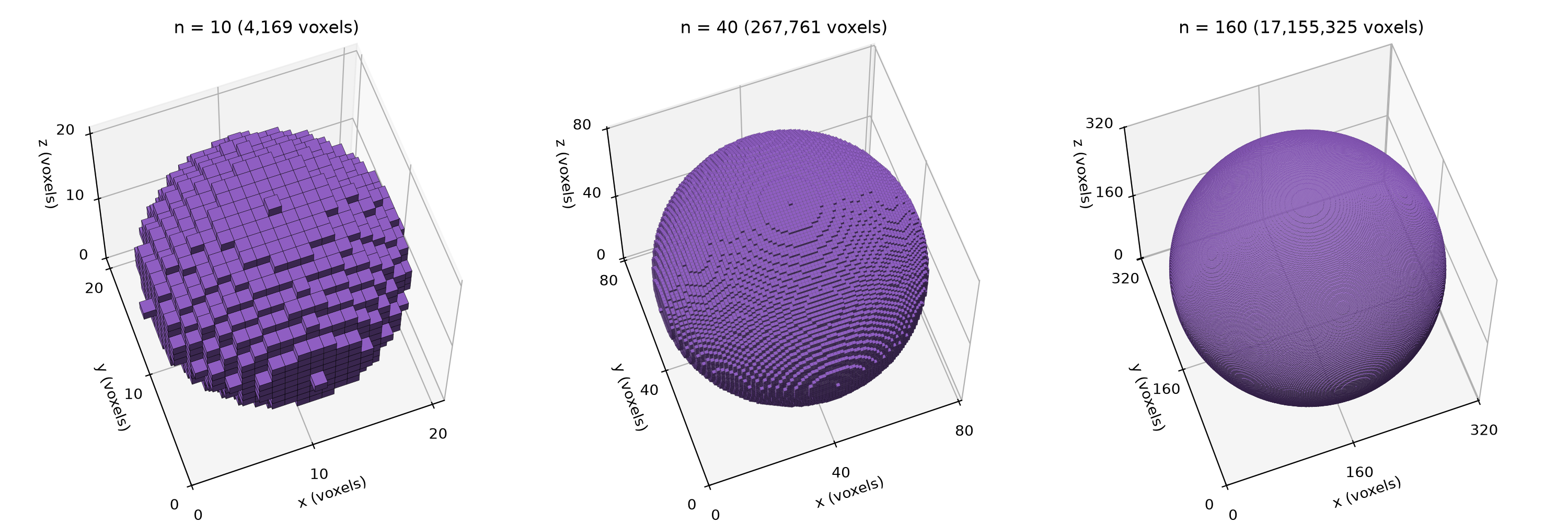
unit_sphere_meshes.py.Marching Cubes
Marching cubes turns a grid of values into a triangulated surface at one
level of those values. The command automesh mesh tri --cubes marching runs
the method of Lewiner et al.1 For each segmentation, automesh
- pads the segmentation by one voxel of zeros, so the surface closes,
- runs marching cubes at level
0.5, halfway between outside (0) and inside (1), - winds every triangle outward, and
- scales and translates the vertices to a unit sphere (see Transform).
The command below meshes the segmentation. The scale is and the translation is in each direction.
automesh mesh tri -i unit_sphere_n010.npy -o unit_sphere_mc_n010.stl --cubes marching \
    --xscale 0.1 --yscale 0.1 --zscale 0.1 \
    --xtranslate -1.05 --ytranslate -1.05 --ztranslate -1.05
The loop below makes the surface for each of the five segmentations.
for n in 10 20 40 80 160; do
  s=$(python3 -c "print(1/$n)")
  t=$(python3 -c "print(-($n + 0.5)/$n)")
  automesh mesh tri -i unit_sphere_n$(printf %03d $n).npy \
    -o unit_sphere_mc_n$(printf %03d $n).stl --cubes marching \
    --xscale $s --yscale $s --zscale $s \
    --xtranslate $t --ytranslate $t --ztranslate $t
done
The surfaces below have the following counts. , , and count the vertices, edges, and faces. The volume is the signed volume that the faces enclose. The error compares that volume with the exact volume .
| volume | error | ||||
|---|---|---|---|---|---|
| 10 | 1,902 | 5,700 | 3,800 | 4.1478 | −0.98% |
| 20 | 7,542 | 22,620 | 15,080 | 4.1699 | −0.45% |
| 40 | 30,150 | 90,444 | 60,296 | 4.1825 | −0.15% |
| 80 | 120,486 | 361,452 | 240,968 | 4.1865 | −0.06% |
| 160 | 482,286 | 1,446,852 | 964,568 | 4.1882 | −0.01% |
The volume created from marching cubes underestimates the true value at every in the table. The surface also encloses less volume than the voxels it came from. This pattern holds at every from 4 to 160. Marching cubes cuts each corner of the voxel staircase with a flat triangle, and every cut removes a small volume.
Five integrity checks run on the five surfaces. All five surfaces give the same result on every check.
- Closed. No edge is open. An open edge belongs to one face only.
- Manifold. No edge is pinched. A pinched edge belongs to more than two faces.
- Oriented. No two faces traverse the same edge in the same direction.
- Connected. The surface is one piece.
- Euler characteristic. .
For a closed, connected, orientable surface, , where is the genus, the number of handles. Here , so , and each surface is topologically a sphere.
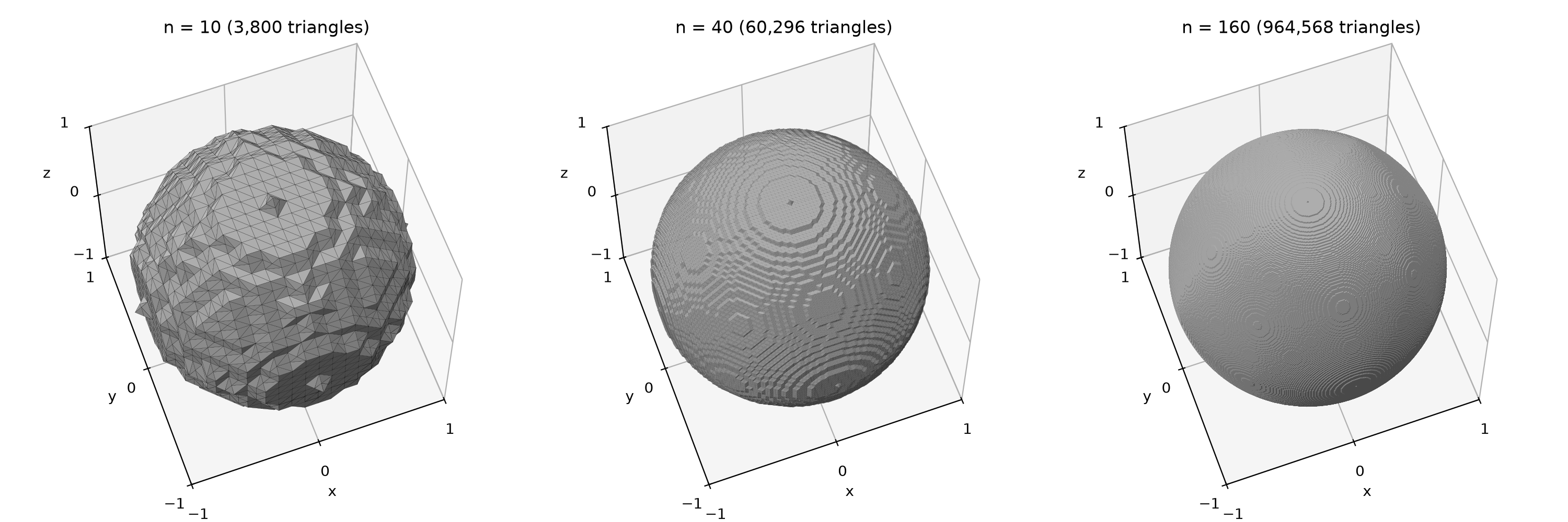
unit_sphere_meshes.py.Convergence
The script
unit_sphere_convergence.py computes both
volumes at every from 4 to 160, 157 values in all. It runs
automesh mesh tri --cubes marching once per .
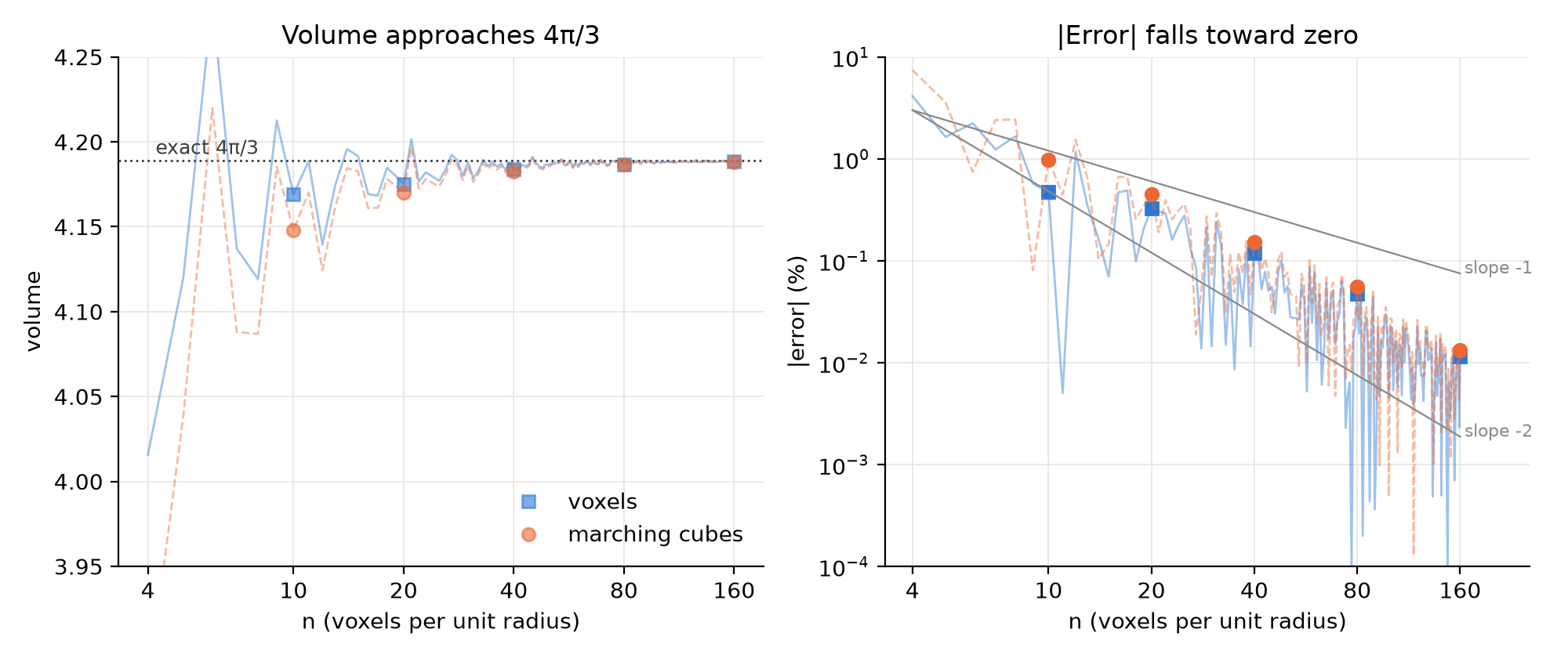
Both volumes settle onto , but neither settles smoothly. The voxel error changes sign 46 times, and 25 of the 157 voxel volumes exceed . The marching cubes error changes sign 24 times, and 12 of its volumes exceed . The five values in the tables just happened to fall short.
Under the oscillation, both errors fall toward zero. A least-squares fit of against gives a slope of −1.71 for the voxels and −1.76 for marching cubes. Both lie between the two guides. The marching cubes volume stays below the voxel volume at all 157 values.
Why Lewiner?
Lorensen and Cline introduced marching cubes in 1987.2 Their method visits each cube of eight neighboring samples. It classifies each corner as inside or outside, which gives 256 cases. Symmetry reduces those to 15 base cases, and each base case has one fixed triangulation.
Some cases are ambiguous. On a face with two inside corners on one diagonal and two outside corners on the other, the corners alone cannot say whether the inside corners connect across the face. An interior ambiguity arises the same way inside a cube. A fixed table picks one answer without looking at the data. Neighboring cubes can then disagree, and the surface can take the wrong topology.
Chernyaev extended the table to 33 cases.3 His table
resolves each ambiguity with the trilinear interpolant of the eight corner
values, the smooth function the samples define inside the cube. Lewiner
et al. gave an efficient and complete implementation of that
table.1 automesh uses the Lewiner method.
The Lewiner method is better than the original table because neighboring cubes always agree. Each ambiguity is resolved from the data, so two cubes that share a face choose the same connection across it. The surface then has the topology of the interpolant's level set.
The sphere reaches no ambiguous case, so the Lewiner method has nothing to resolve here, and no edge of the surface is pinched at any . On data that do reach such cases, the original table can return a surface of different topology. Newman and Yi illustrate each ambiguous case and survey the methods that resolve them.4
A binary mask needs one further caution. On a mask of 0 and 1, the level 0.5 is
exactly the saddle value of an ambiguous face. At that tie, the Lewiner method
can pinch an edge between four faces. automesh uses the level 0.5. The
sphere is a special case that never reaches the tie.
Transform
Marching cubes returns vertices in voxel units. Voxel spans , so the voxel at index spans . That voxel is the center of the sphere, so the center sits at its midpoint, . Two operations map the surface to a unit sphere at the origin.
- Scale by , which makes the radius 1.
- Translate by , which moves the center to the origin.
The --xscale and --xtranslate options of automesh scale first and
translate second, in that order. The translation must use . A
translation of treats the center as the upper face of voxel ,
at . It leaves the surface off center by in each direction.
The vertex radii show how close the surface comes to the unit sphere. The coefficient of variation, CoV , measures how much the radii spread. A perfect sphere has CoV .
| min | max | mean | CoV | |
|---|---|---|---|---|
| 10 | 0.9552 | 1.0500 | 0.9993 | 2.15% |
| 20 | 0.9763 | 1.0250 | 0.9991 | 1.01% |
| 40 | 0.9878 | 1.0125 | 0.9996 | 0.51% |
| 80 | 0.9938 | 1.0063 | 0.9999 | 0.26% |
| 160 | 0.9969 | 1.0031 | 1.0000 | 0.13% |
The mean radius stays within 0.1% of 1 at every , so a scale of leaves no bias. The largest radius is always , at the six poles. There a vertex sits halfway between the last inside voxel, at radius , and the first outside voxel, at radius .
The CoV halves each time doubles, so the spread of the radii falls as . That is first order, slower than the volume error in Convergence. The volume averages over the whole surface, and the staircase steps partly cancel in that average. The radius spread sees every step.
Surface Comparison
Hausdorff Distance
The Hausdorff distance between two surfaces is the farthest that any point of either one lies from the other. For a surface and the unit sphere ,
The script unit_sphere_comparison.py computes the
first term exactly. A point lies from
the unit sphere. Over a triangle, is convex. Its largest value sits at
a vertex, and its smallest sits at the point of the triangle closest to the
origin.5 The largest over all triangles gives the
outward distance. The largest gives the inward distance.
The second term needs no computation. Each surface is closed and encloses the origin. The ray from the origin through a sphere point therefore crosses at some point . Then . The second term never exceeds the first, so the Hausdorff distance is the larger of the outward and inward distances.
uv run --with numpy unit_sphere_comparison.py
| outward | inward | ||||
|---|---|---|---|---|---|
| 10 | 3,800 | 0.05000 | 0.04737 | 0.05000 | 0.500 |
| 20 | 15,080 | 0.02500 | 0.02436 | 0.02500 | 0.500 |
| 40 | 60,296 | 0.01250 | 0.01234 | 0.01250 | 0.500 |
| 80 | 240,968 | 0.00625 | 0.00621 | 0.00625 | 0.500 |
| 160 | 964,568 | 0.00312 | 0.00312 | 0.00312 | 0.500 |
The Hausdorff distance is exactly at every , half a voxel. The outward distance sets it, at the six poles (see Transform). The inward distance approaches it from below. The Hausdorff distance falls as , first order, like the radius CoV. The triangle count grows as , so in terms of triangles the distance falls only as .
Surface Area
The volume converges, as the Convergence section shows. The
surface area does not converge. The script
unit_sphere_comparison.py adds up the areas of
the marching cubes triangles. The error compares that area with the exact
area .
| area | error | |
|---|---|---|
| 10 | 13.7204 | +9.18% |
| 20 | 13.6324 | +8.48% |
| 40 | 13.6566 | +8.68% |
| 80 | 13.6608 | +8.71% |
| 160 | 13.6673 | +8.76% |
The voxel staircase itself would overstate the area by 50% at any . Marching cubes cuts the voxel staircase corners, which removes most of that excess. Howver, the surface area still settles near 8.8% too large.
Smaller voxels make smaller steps, but the triangles keep the same few orientations relative to the true surface. So the Hausdorff distance falls to zero while the area error does not. A surface can come arbitrarily close to the sphere and still have the wrong area.
Triangle Quality
The script unit_sphere_comparison.py also runs
automesh metrics on each surface. The
Triangular Metrics page defines its
measures.
A binary mask puts every vertex at the midpoint of a cube edge. So marching cubes can make only a few triangle shapes. Grouped by maximum edge ratio and minimum scaled Jacobian, the triangular surfaces created by marching cubes produce exactly five shapes. The table gives the fraction of triangles of each shape.
| shape | angles | edge ratio | scaled Jacobian | |||||
|---|---|---|---|---|---|---|---|---|
| equilateral | 60°, 60°, 60° | 1.000 | 1.000 | 14.74% | 14.80% | 14.30% | 13.99% | 13.98% |
| right isosceles | 45°, 45°, 90° | 1.414 | 0.816 | 24.63% | 25.15% | 25.04% | 24.92% | 24.85% |
| right | 35.26°, 54.74°, 90° | 1.732 | 0.667 | 31.58% | 30.56% | 32.08% | 33.13% | 33.20% |
| obtuse isosceles | 30°, 30°, 120° | 1.732 | 0.577 | 14.53% | 14.75% | 14.29% | 13.98% | 13.98% |
| 30-60-90 | 30°, 60°, 90° | 2.000 | 0.577 | 14.53% | 14.75% | 14.29% | 13.98% | 13.98% |
Refinement does not change the quality. The same five shapes appear at every , in nearly the same proportions. More than a quarter of the triangles have the worst scaled Jacobian, , with a smallest angle of 30°. No triangle is worse.
Smaller voxels shrink the triangles but never reshape them. A histogram of any measure would show only these five spikes, so the table is shown instead of a histogram.
Mesh
Sculpt
The Subdivision page meshes its Octa-Loop spheres with Sculpt. At levels 3 to 7, it reports a grid of 26×26×26 cells, 7,731 nodes, and 6,672 elements. Here Sculpt meshes the marching cubes surfaces on the same grid.
The Subdivision baseline runs Sculpt through Cubit's sculpt parallel
command, which chooses the grid itself. For Octa-Loop level 3, Cubit places 26
cells in each direction across a box of , a cell size of about
0.0954. Standalone Sculpt with those options reproduces the baseline exactly,
at 7,731 nodes and 6,672 elements. The same options mesh each marching cubes
surface.
B=1.240409
GRID="-x 26 -y 26 -z 26 -t -$B -u -$B -v -$B -q $B -r $B -s $B -SS 2"
# octa_loop03.stl downloads from the Refinement table of the Subdivision page
sculpt -j 1 -stl octa_loop03.stl $GRID -e unit_sphere_sculpt_octa03
for n in 010 020 040 080 160; do
  sculpt -j 1 -stl unit_sphere_mc_n$n.stl $GRID -e unit_sphere_sculpt_n$n
done
Left to choose its own grid, Cubit sizes the cells to the small marching cubes facets. For it picks 73×73×73 cells and makes 180,201 elements. Fixing the grid keeps the meshes comparable with the baseline.
The quality is the minimum scaled Jacobian, as Sculpt reports it.
| input | nodes | elements | minimum quality | mean quality |
|---|---|---|---|---|
| Octa-Loop level 3 (baseline) | 7,731 | 6,672 | 0.343 | 0.888 |
| marching cubes, | 8,007 | 6,912 | 0.388 | 0.885 |
| marching cubes, | 7,827 | 6,768 | 0.404 | 0.900 |
| marching cubes, | 7,827 | 6,768 | 0.420 | 0.902 |
| marching cubes, | 7,827 | 6,768 | 0.401 | 0.901 |
| marching cubes, | 7,827 | 6,768 | 0.427 | 0.901 |
From on, every surface gives the same 7,827 nodes and 6,768 elements, 96 more of each than the baseline, or about 1.4%. The worst element is better than the baseline's at every .
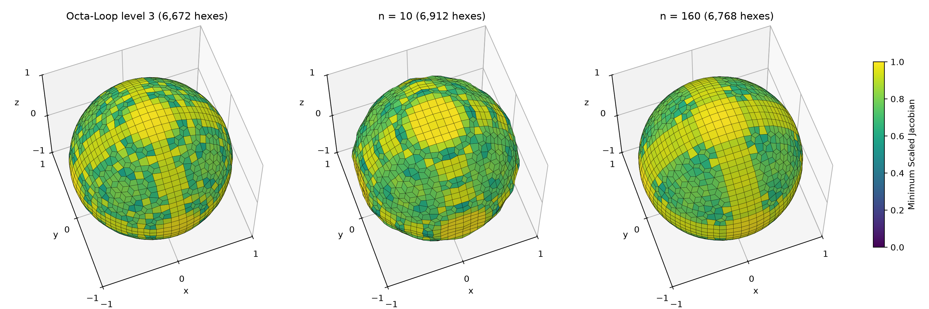
unit_sphere_meshes.py.The difference between the middle and right panels comes from the size of a voxel step against the size of a Sculpt cell, about 0.095.
- At , a voxel is 0.1 wide, so each step is about as large as a cell. The mesh boundary follows the steps, and the sphere looks lumpy.
- At , a voxel is 0.00625 wide, so a cell spans about 15 voxels. The steps are far smaller than the elements, and the mesh looks like the baseline.
- From on, a cell spans about two voxels or more, and the mesh stops changing.
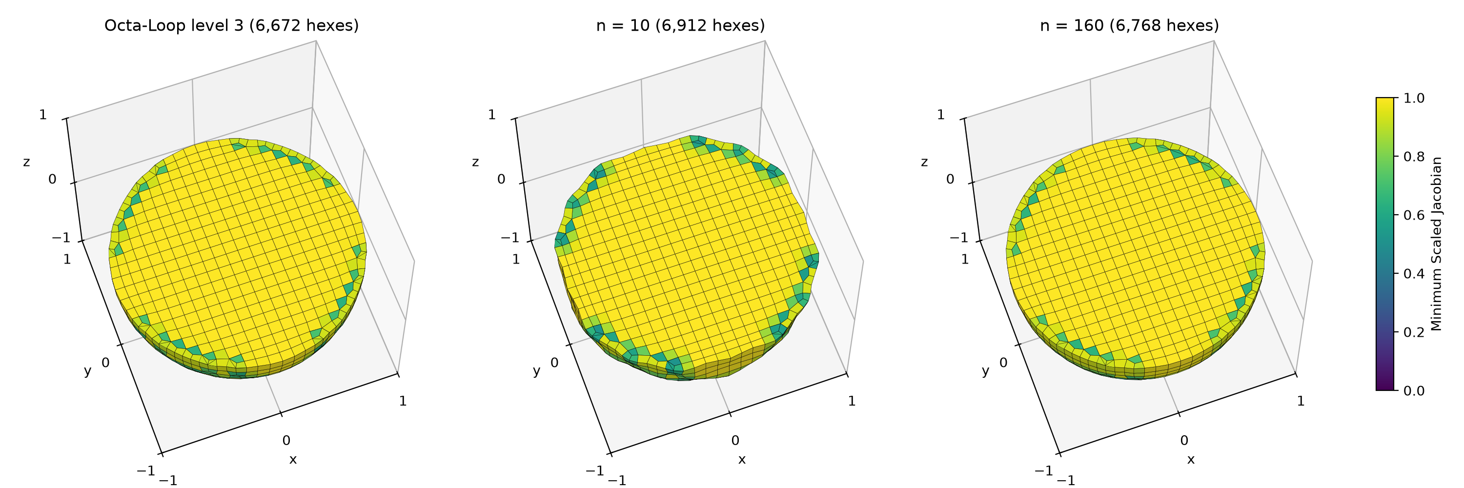
unit_sphere_meshes.py.The run used Sculpt 16.08, from Cubit 16.08. The files unit_sphere_sculpt_*.e.1.0
are Sculpt outputs, and the repository does not contain them. The scripts of
this page read them from this directory, so regenerating the Sculpt figures and
table requires running the Sculpt commands above. automesh reads Sculpt's Exodus
files directly, and automesh metrics gives the same minimum (0.343) and mean
(0.888) as Sculpt for the baseline mesh.
automesh
automesh mesh hex meshes the marching cubes surface in two ways.
The uniform mesh uses the Sculpt cell size, , so its lattice matches the Sculpt grid. The adaptive mesh uses the
defaults.
automesh mesh hex -i unit_sphere_mc_n010.stl -o uniform.inp \
  -u 0.095416 --metrics uniform.csv
automesh mesh hex -i unit_sphere_mc_n010.stl -o adaptive.inp \
  --metrics adaptive.csv
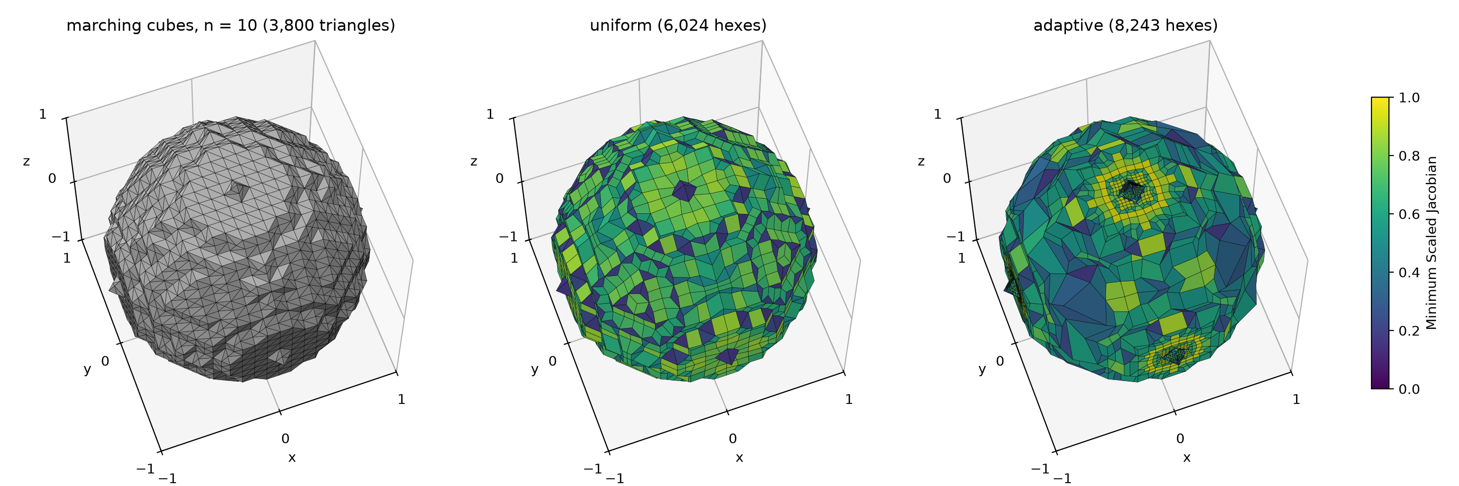
unit_sphere_mc_n010.stl, (center) automesh uniform, (right) automesh adaptive.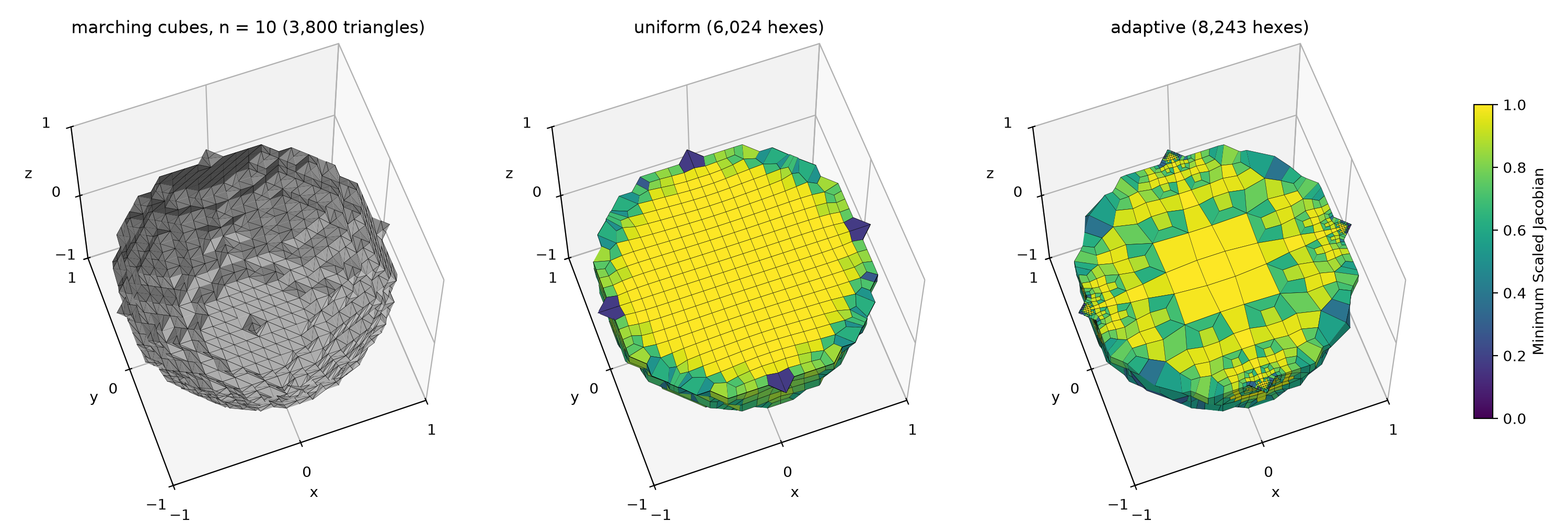
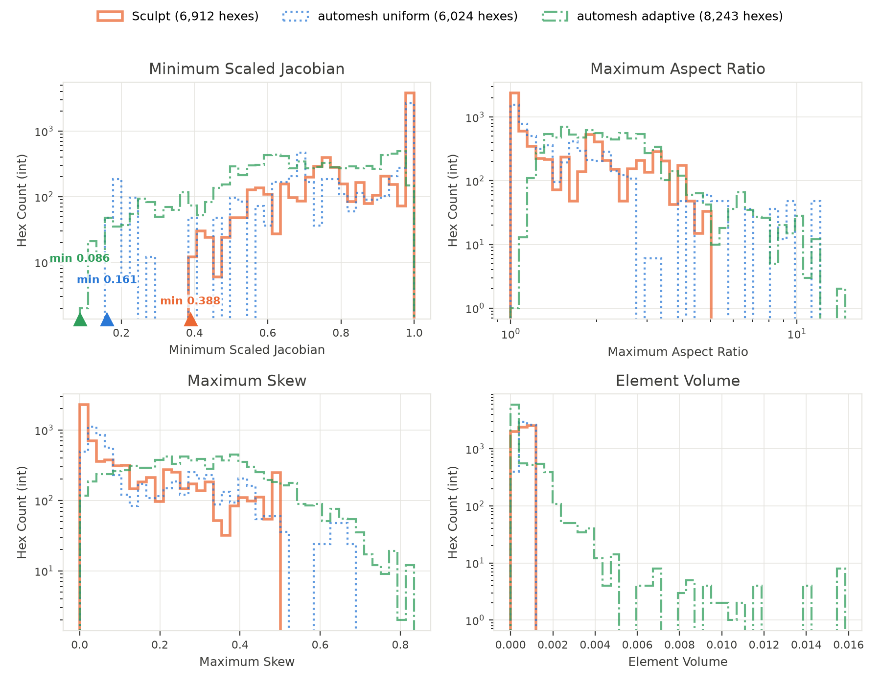
automesh uniform and adaptive, both without prior smoothing of the marching cubes surface.Taubin Smoothing
Taubin smoothing rounds the voxel steps of the surface. This section measures how the number of smoothing iterations changes the Minimum Scaled Jacobian of the uniform and adaptive meshes.
automesh smooth applies Taubin smoothing with its defaults. The pass band is
0.1 and the scale is , which gives . Each
iteration is one Laplacian step. Odd-numbered iterations shrink the surface
with . Even-numbered iterations inflate it with . The sweep runs
every integer from 0 to 100 iterations, every tenth from 110 to 300, and every
fiftieth from 350 to 1,000. Each smoothed surface gets a uniform mesh with the
Sculpt cell size and an adaptive mesh with the defaults.
automesh smooth -i unit_sphere_mc_n010.stl -o smooth.stl --iterations 260
automesh mesh hex -i smooth.stl -o uniform.inp -u 0.095416 --metrics uniform.csv
automesh mesh hex -i smooth.stl -o adaptive.inp --metrics adaptive.csv
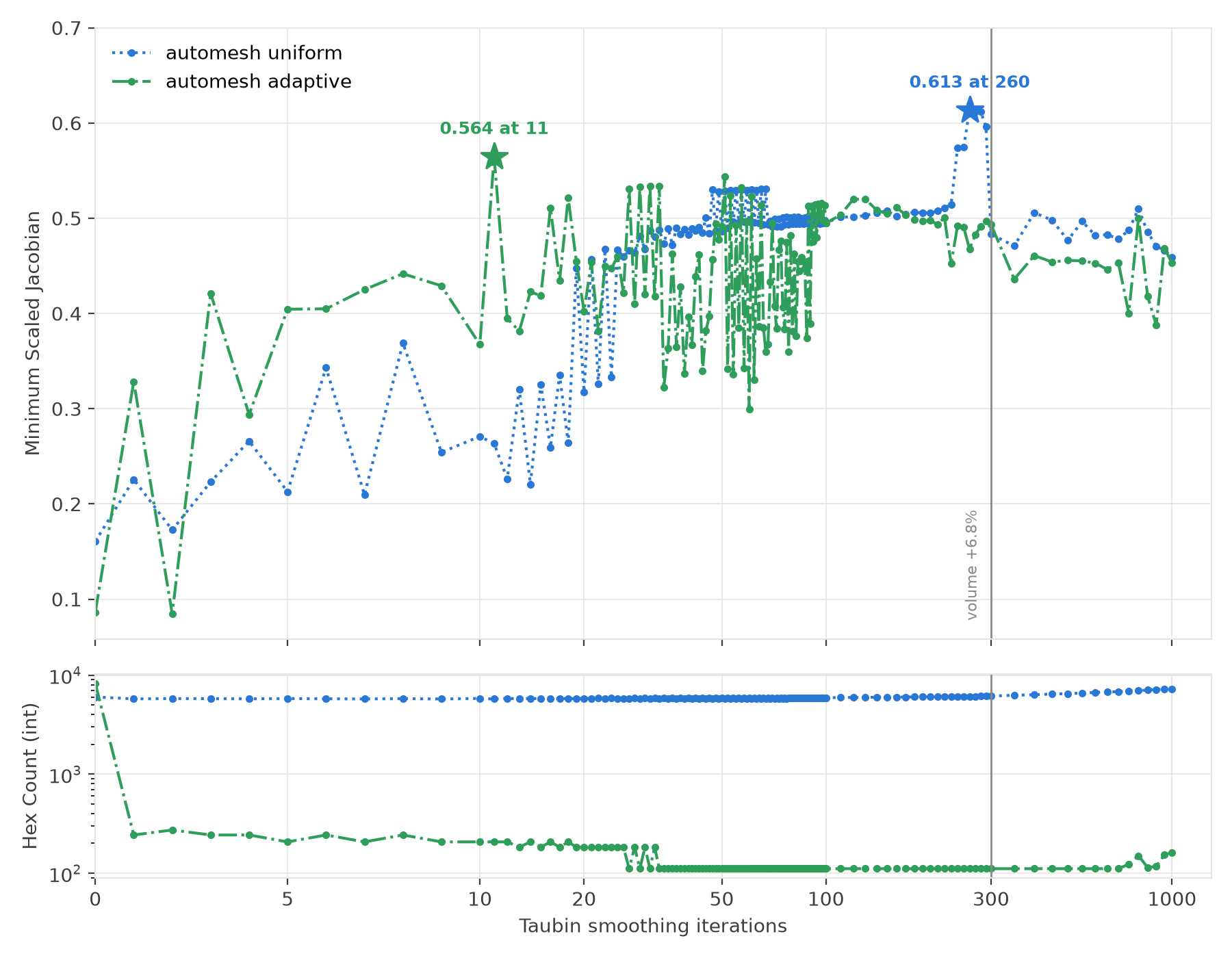
automesh uniform and adaptive meshes of the surface, against the number of Taubin smoothing iterations. Stars mark the peak of each series up to 300 iterations. Each peak is also the highest value of the whole sweep. The vertical line at 300 iterations marks a surface volume 6.8% above the sphere's. The x-axis is linear to 10 iterations and logarithmic beyond.Uniform. The minimum rises with scatter from 0.161 at 0 iterations to 0.613 at 260 iterations. The mean rises from 0.827 to 0.901. Up to 300 iterations the hex count stays between 5,747 and 6,150, against 6,024 without smoothing. The peak is a plateau: 0.613, 0.612, and 0.612 at 260, 270, and 280 iterations, against 0.574 and 0.575 at 240 and 250. The minimum then falls to 0.483 at 300 iterations and scatters between 0.459 and 0.510 up to 1,000.
Adaptive. The hex count falls from 8,243 at 0 iterations to 243 at 1 iteration. From 34 to 700 iterations it stays at 111 hexes. The minimum peaks at 0.564 at 11 iterations, on 207 hexes. The peak is a spike, not a plateau. The minimum is 0.367 at 10 iterations and 0.395 at 12. The next highest minimum is 0.544 at 51 iterations, on 111 hexes. The 111-hex meshes start at 0.323 at 34 iterations and scatter between 0.299 and 0.544 up to 700.
Surface drift. The defaults inflate this surface, because exceeds . The mean vertex radius grows from 0.9992 at 0 iterations to 1.0207 at 260 and 1.0862 at 1,000. The enclosed volume is 4.126 at 11 iterations, 1.5% below . It is 4.428 at 260 iterations, 5.7% above, and 5.322 at 1,000, 27.1% above. The peak search therefore stops at 300 iterations.
Odd and even counts. An odd count ends on a shrink step and an even count on an inflate step, so neighboring counts give different surfaces. The enclosed volume is 4.115 at 1 iteration and 4.149 at 2. The adaptive minimum is 0.328 at 1 iteration and 0.085 at 2. The uniform minimum is 0.223 at 3 iterations and 0.266 at 4.
None of the 270 meshes has an inverted hex.
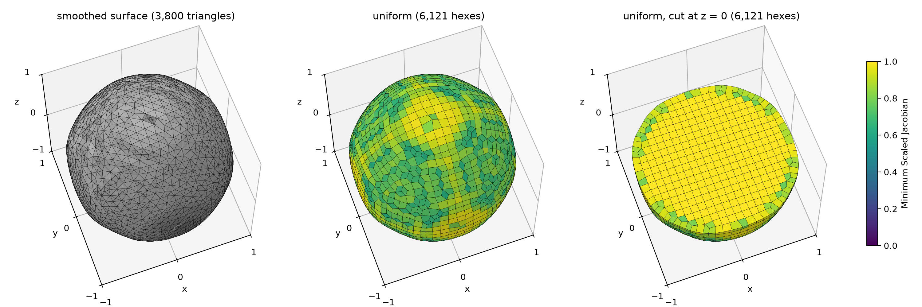
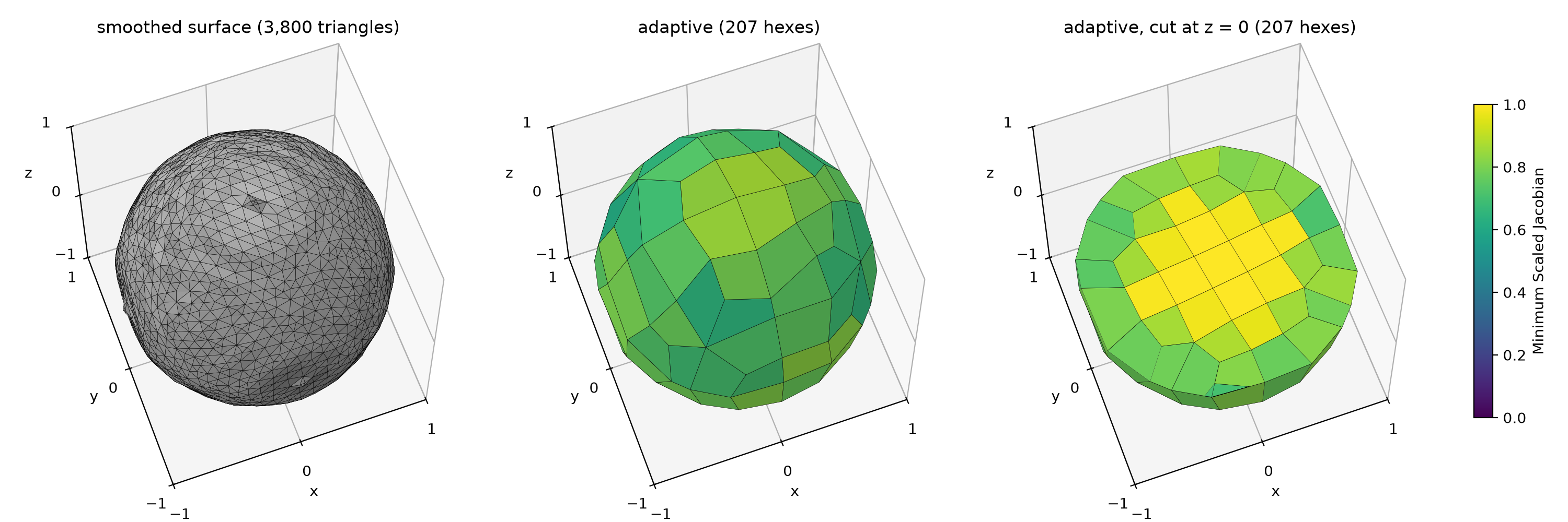
Quality After Smoothing
The figure below compares the two best meshes of the sweep with the same meshes before smoothing and with the Sculpt baseline. The uniform mesh comes from the surface smoothed 260 times, with a minimum of 0.613. The adaptive mesh comes from the surface smoothed 11 times, with a minimum of 0.564. Without smoothing, the minima are 0.161 and 0.086. The Sculpt minimum is 0.388.
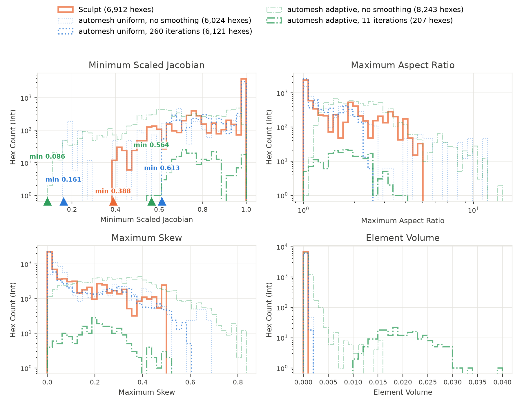
automesh uniform mesh after 260 Taubin smoothing iterations and the adaptive mesh after 11, the best Minimum Scaled Jacobian of each, against the same meshes without smoothing (faint lines) and the Sculpt mesh for . The figure is produced by unit_sphere_smooth.py.| input | nodes | elements | minimum quality | mean quality |
|---|---|---|---|---|
| Octa-Loop level 3 (baseline) | 7,731 | 6,672 | 0.343 | 0.888 |
| marching cubes, | 8,007 | 6,912 | 0.388 | 0.885 |
| automesh uniform, before smoothing | 7,035 | 6,024 | 0.161 | 0.827 |
| automesh adaptive, before smoothing | 10,016 | 8,243 | 0.086 | 0.694 |
| automesh uniform, best result with smoothing (260 iterations) | 7,120 | 6,121 | 0.613 | 0.901 |
| automesh adaptive, best result with smoothing (11 iterations) | 288 | 207 | 0.564 | 0.793 |
The quality is the minimum scaled Jacobian, as in the Sculpt table. The first two rows, the Sculpt meshes of the Sculpt section, are the reference. Smoothing raises the uniform minimum from 0.161 to 0.613 and the adaptive minimum from 0.086 to 0.564. Of the two best meshes, the uniform mesh has the higher minimum, by 0.049, and the higher mean, by 0.108.
The adaptive mesh has 207 hexes, 3.4% of the uniform count, so its histograms sit about a factor of 30 lower. Compare the shapes of the curves, not their heights.
The two minima differ in how robust they are. The uniform value belongs to a plateau: 0.613, 0.612, and 0.612 at 260, 270, and 280 iterations. The adaptive value belongs to a spike: 0.367 at 10 iterations, 0.564 at 11, and 0.395 at 12. A small change in the iteration count would lose the adaptive result.
Remesh
automesh remesh replaces the triangles of a surface
with near-equilateral triangles of one target edge length. The marching
cubes surface has 3,800 triangles. Their edge lengths range from 0.071 to 0.141,
and the worst angle is 30.0°. This section remeshes the surface to the mean edge
length of Octa-Loop level 4, 0.1178, the smooth control surface of the
Control Study below.
Two runs follow. The first remeshes the surface alone. The second smooths the
surface with 20 Taubin iterations, remeshes it, and smooths it again with 20
iterations. Every automesh smooth call uses its defaults: 20 iterations, a
Taubin scale of 0.6307, and a pass band of 0.1. The 20 remesh iterations are a
test value. They are not an optimum.
In a trial outside unit_sphere_remesh.py, five orders of smoothing and
remeshing used 20 iterations in every step. Smoothing before and after the
remesh gave the lowest radius RMS, defined below the figure: 0.00688, against
0.00739 to 0.00903 for the other four.
automesh remesh -i unit_sphere_mc_n010.stl -o remesh.stl \
  uniform --iterations 20 --size 0.1178
automesh smooth -i unit_sphere_mc_n010.stl -o smooth.stl --iterations 20
automesh remesh -i smooth.stl -o smooth_remesh.stl \
  uniform --iterations 20 --size 0.1178
automesh smooth -i smooth_remesh.stl -o smooth_remesh_smooth.stl --iterations 20
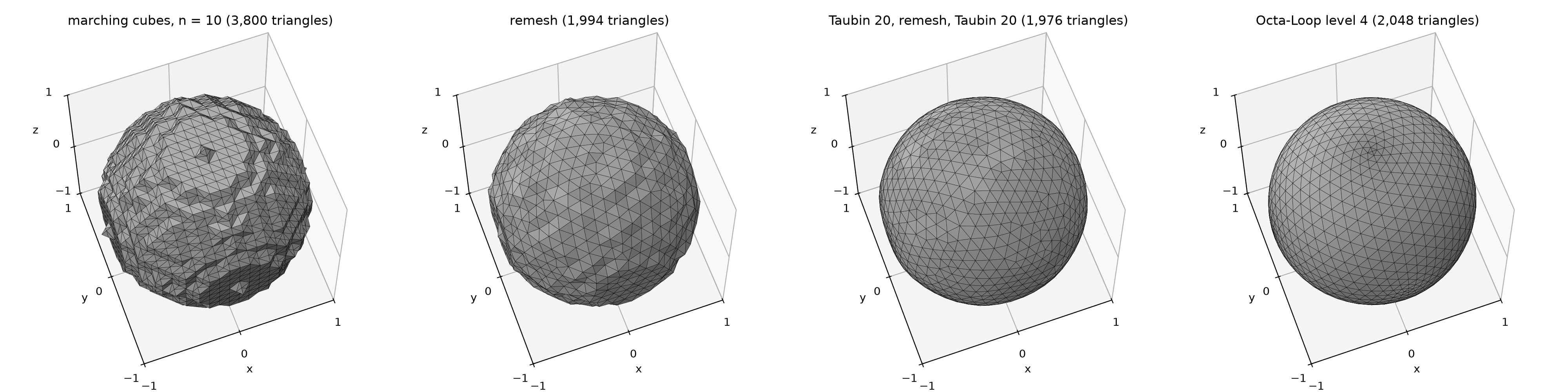
unit_sphere_remesh.py.| surface | triangles | edge length CoV | minimum angle | vertex radius | radius RMS | maximum / RMS dihedral angle | area | volume | |
|---|---|---|---|---|---|---|---|---|---|
| marching cubes, | 3,800 | 0.262 | 30.0° | 0.955–1.050 | 0.02150 | 0.0500 | 70.5° / 24.9° | 13.720 | 4.148 |
| remesh | 1,994 | 0.090 | 42.1° | 0.954–1.035 | 0.01779 | 0.0463 | 54.0° / 17.2° | 12.884 | 4.123 |
| Taubin 20, remesh, Taubin 20 | 1,976 | 0.096 | 42.8° | 0.973–1.011 | 0.00688 | 0.0269 | 11.1° / 4.5° | 12.576 | 4.181 |
| Octa-Loop level 4 | 2,048 | 0.142 | 45.0° | 0.998–1.003 | 0.00158 | 0.0034 | 4.7° / 4.0° | 12.521 | 4.162 |
The exact sphere has area and volume . Every surface is closed. The coefficient of variation (CoV) of the edge length is , the standard deviation of the edge lengths divided by their mean. It is 0 when every edge has the same length.
The radius of a vertex is its distance from the origin, so a vertex on the unit sphere has . The radius RMS is the root mean square of over the vertices. It is the typical distance of a vertex from the unit sphere, whether the vertex lies inside or outside. The dihedral angle of an edge is the angle between the normals of its two triangles. It is 0° where the two triangles lie in one plane. The table lists the maximum and the root mean square of the dihedral angle over the edges.
Remesh alone. Remeshing cuts the triangle count from 3,800 to 1,994. It cuts the coefficient of variation of the edge length from 0.262 to 0.090. It raises the worst angle from 30.0° to 42.1°. It does not round the steps. The vertex radius still ranges from 0.954 to 1.035, against 0.955 to 1.050 before. The radius RMS is 0.01779, against 0.02150 before, and the maximum dihedral angle is 54.0°, against 70.5°. The area falls from 13.720 to 12.884, still 2.5% above .
Smooth, remesh, smooth. Twenty Taubin iterations before the remesh round the steps. Twenty more after the remesh round what the remesh leaves. The radius RMS falls to 0.00688, from 0.01779 for the remesh alone. The largest falls from 0.0463 to 0.0269. The maximum dihedral angle falls from 54.0° to 11.1°, and its RMS from 17.2° to 4.5°. The area is 12.576, 0.08% above . The volume is 4.181, 0.19% below . The surface has 1,976 triangles, a coefficient of variation of 0.096, and a worst angle of 42.8°.
Against Octa-Loop level 4. Octa-Loop level 4 has 2,048 triangles, a coefficient of variation of 0.142, a worst angle of 45.0°, a radius RMS of 0.00158, a largest of 0.0034, and dihedral angles of 4.7° at most and 4.0° RMS. The smoothed and remeshed surface has the lower coefficient of variation, by 0.046. Its worst angle is 2.2° smaller. Its radius RMS is 4.4 times that of Octa-Loop level 4, its largest is about 8 times, and its maximum dihedral angle is 2.4 times. Its RMS dihedral angle is 0.5° higher.
Edge lengths. The surface has four distinct edge lengths, shared among its 5,700 edges:
- 0.0707 on 39.8% of the edges,
- 0.1000 on 26.9%,
- 0.1225 on 20.2%, and
- 0.1414 on 13.1%.
Remeshing spreads them over a range: 0.090 to 0.159 after remeshing, and 0.092 to 0.155 after smoothing, remeshing, and smoothing. The mean edge length is 0.122 after remeshing and 0.121 after the three steps, against the target of 0.1178. The share of edges within 10% of the target is 20.2% for the marching cubes surface, 67.3% after remeshing, and 66.4% after the three steps.
Octa-Loop level 4 has 57.0% of its edges within 10% of the target, below both remeshed surfaces. It has a tail of short edges. Its shortest edge is 0.045 and its 5th percentile is 0.083, against 0.092 and 0.100 for the smoothed and remeshed surface. Its longest edge is 0.134, against 0.155.
Control Study
automesh mesh hex's adaptive octree combines two refinement signals:
- curvature-driven sizing, gated by a chord-error tolerance
(
--tolerance, disabled by default), and - local-thickness sizing, from the shape diameter function of Shapira, Shamir, and Cohen-Or.6
No script on this page passes --tolerance, so curvature-driven sizing never
activates here. Local thickness alone (not curvature) sets the octree's
refinement target.
Taubin smoothing raised the Minimum Scaled Jacobian of the marching cubes
meshes, from 0.161 to 0.613 for the uniform mesh and from 0.086 to 0.564 for the
adaptive mesh. The control study asks whether a surface that is already smooth
does better than that. The control is Octa-Loop level 4, a Loop subdivision of
an octahedron from the Subdivision
page. Its file, octa_loop04.stl, downloads from the Refinement table. The
surface is closed, has 2,048 triangles, and its 1,026 vertices lie within 0.3% of
the unit sphere.
Level 4 is the level whose triangle count is closest to that of the smoothed surface. Smoothing moves the vertices and leaves the count at 3,800. Level 3 has 512 triangles, level 4 has 2,048, and level 5 has 8,192. The mean triangle edge points the same way: 0.118 for level 4 against 0.092 for the smoothed surface, and about 0.059 for level 5, since each level halves the edge.
automesh mesh hex -i octa_loop04.stl -o octa_uniform.inp \
  -u 0.095416 --metrics octa_uniform.csv
automesh mesh hex -i octa_loop04.stl -o octa_adaptive.inp \
  --metrics octa_adaptive.csv
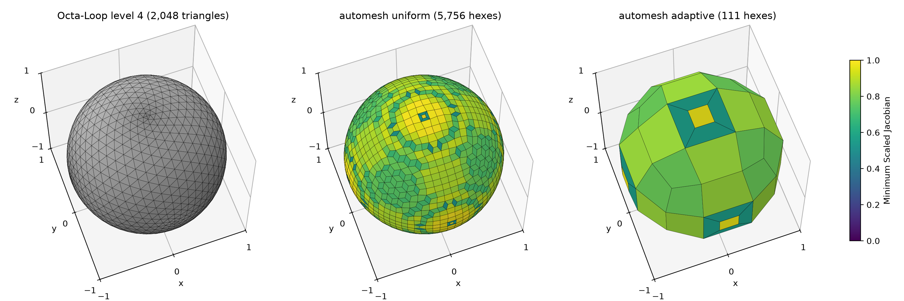
octa_loop04.stl (2,048 triangles), (center) automesh uniform (5,756 hexes), (right) automesh adaptive (111 hexes).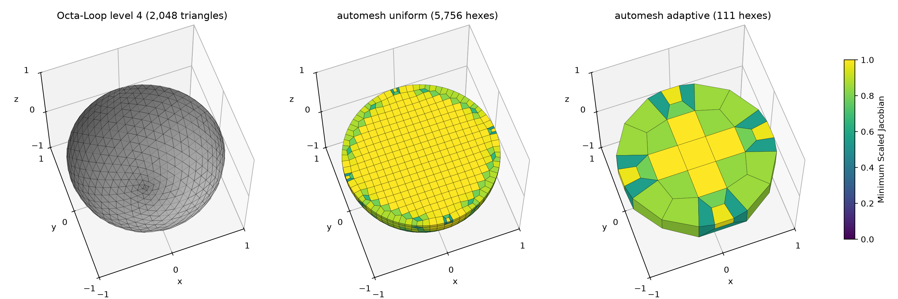
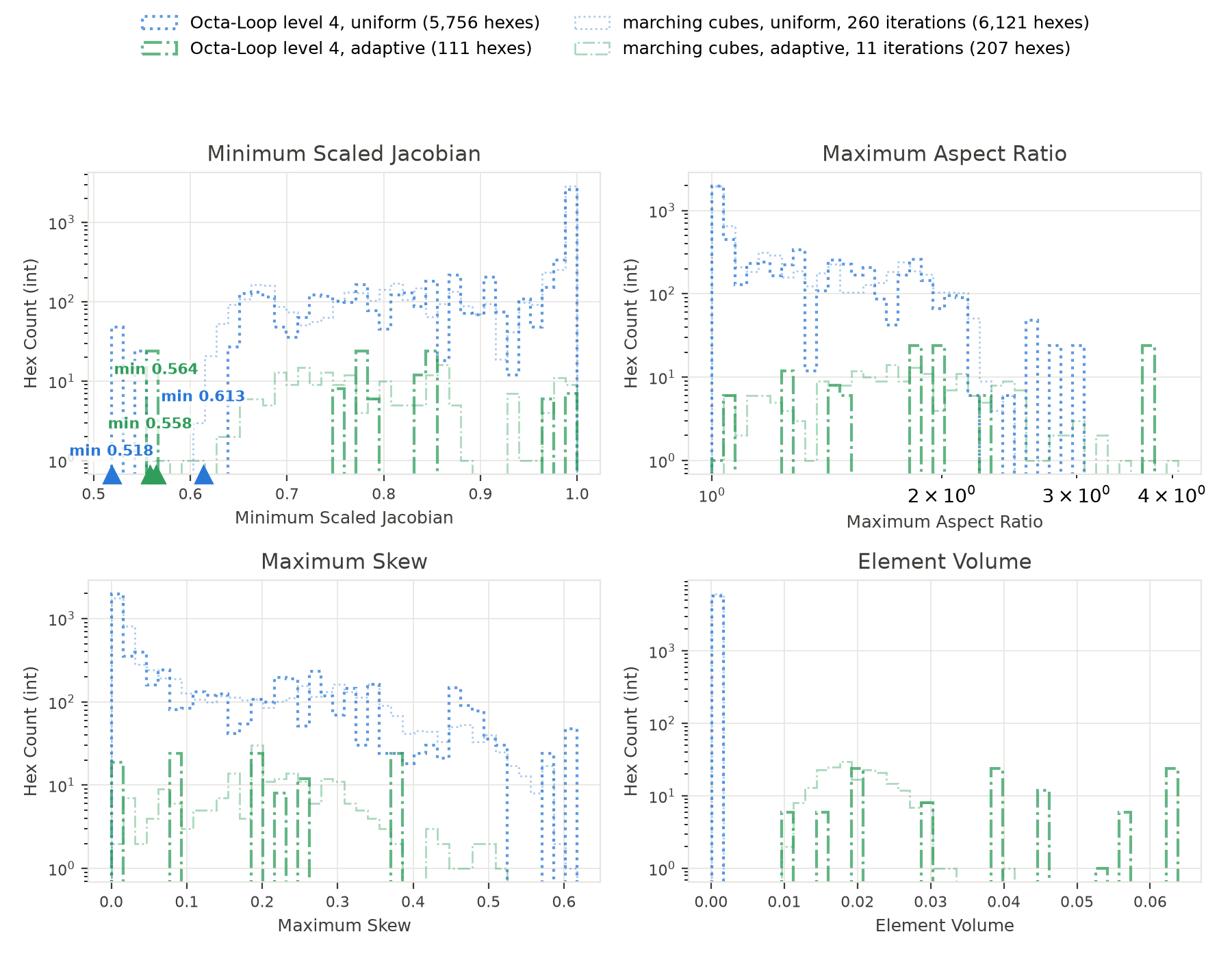
automesh uniform and adaptive meshes of Octa-Loop level 4, against the best Taubin-smoothed marching cubes meshes of the previous section (faint lines). The figure is produced by unit_sphere_control.py.| input | nodes | elements | minimum quality | mean quality |
|---|---|---|---|---|
| marching cubes, uniform, best result with smoothing (260 iterations) | 7,120 | 6,121 | 0.613 | 0.901 |
| marching cubes, adaptive, best result with smoothing (11 iterations) | 288 | 207 | 0.564 | 0.793 |
| Octa-Loop level 4, uniform | 6,737 | 5,756 | 0.518 | 0.903 |
| Octa-Loop level 4, adaptive | 168 | 111 | 0.558 | 0.775 |
The smooth surface does not beat the best smoothed surface. The uniform mesh of Octa-Loop level 4 has a minimum of 0.518, which is 0.095 below the best smoothed marching cubes mesh, and a mean of 0.903, which is 0.002 above it. The adaptive mesh has a minimum of 0.558, 0.006 below, and a mean of 0.775, 0.018 below. The adaptive mesh has 111 hexes, against 207.
The comparison favors the smoothed surface, because its result is the maximum of 135 iteration counts and the Octa-Loop result is one run. Only 17 of the 135 counts give a uniform minimum above 0.518. Only 1 gives an adaptive minimum above 0.558, the best one itself. From 100 iterations on, the median minimum is 0.503 for the uniform mesh and 0.492 for the adaptive mesh, and the Octa-Loop values are above both. Against the unsmoothed marching cubes meshes, the Octa-Loop minima are 0.518 against 0.161 for the uniform mesh and 0.558 against 0.086 for the adaptive mesh.
A smooth input surface reaches, in one run and with no search over iteration counts, a minimum within 0.006 of the best smoothed adaptive result, and 0.095 below the best smoothed uniform result. None of the four meshes has an inverted hex.
-
Thomas Lewiner, Hélio Lopes, Antônio Wilson Vieira, and Geovan Tavares. "Efficient implementation of Marching Cubes' cases with topological guarantees." Journal of Graphics Tools 8(2) (2003) 1–15. https://doi.org/10.1080/10867651.2003.10487582 ↩ ↩2
-
William E. Lorensen and Harvey E. Cline. "Marching cubes: A high resolution 3D surface construction algorithm." ACM SIGGRAPH Computer Graphics 21(4) (1987) 163–169. https://doi.org/10.1145/37402.37422 ↩
-
Evgeni V. Chernyaev. Marching Cubes 33: Construction of topologically correct isosurfaces. Technical Report CN/95-17, CERN, 1995. ↩
-
Timothy S. Newman and Hong Yi. "A survey of the marching cubes algorithm." Computers & Graphics 30(5) (2006) 854–879. https://doi.org/10.1016/j.cag.2006.07.021 ↩
-
Christer Ericson. Real-Time Collision Detection. Morgan Kaufmann, 2005. Section 5.1.5, the closest point on a triangle to a point. ↩
-
Lior Shapira, Ariel Shamir, and Daniel Cohen-Or. "Consistent mesh partitioning and skeletonisation using the shape diameter function." The Visual Computer 24 (2008) 249–259. https://doi.org/10.1007/s00371-007-0197-5 ↩
Representative Volume Element (RVE)
A heterogeneous material varies in its composition from point to point. A Representative Volume Element (RVE) is the smallest sample volume that still captures the bulk behavior. It reproduces the average physical and mechanical properties of the whole material.
This example uses a unit cube of bulk material. Three spherical pores sit in the interior. Cubit creates the geometry and the tetrahedral comparison meshes; see References for the journal file and Downloads for the files themselves.
Figure 5.1.2-1: The RVE geometry. Left: the solid unit cube. Right: the same model
cut at the plane , which exposes all three pores. The pores have radii
R/10, R/20, and R/30, and only the middle one sits at the origin. Their
centers are collinear and all lie on the cut plane, so each pore is sliced
through its center and appears as an exact circle. The figure is produced by
rve_geometry_figure.py.
Cubit creates the tessellated surface comparison.stl, illustrated below.
Figure 5.1.2-2: The comparison.stl surface, as exported by Cubit. Left: the full
surface triangulation. Right: the interior pore surfaces on their own, drawn
inside a wireframe of the cube. The journal exports the STL before meshing, so
this is the geometry faceting rather than a mesh. The six planar cube faces
need only two triangles each, which puts 3,264 of the total 3,276 facets on
the three pores. The figure is produced by rve_figures.py.
Motivation
The existing approach meshes the RVE with tet4 or tet10 elements. The tet4 mesh appears in the Metrics figure below. The tet10 mesh is not shown separately: its corner nodes reproduce the tet4 mesh exactly, so the two are indistinguishable in a surface view.
The two tetrahedral meshes share the same 35,457 elements. The tet10 mesh adds a midside node on every edge, which raises the node count without changing the topology.
We would like to replace the incumbent tet4/tet10 approach with an adaptive,
all-hexahedral mesh from automesh. The automesh hex mesh needs about half
as many elements as the tet4 mesh. Its node count falls between the two
tetrahedral meshes.
| model | tet4 | tet10 | hex |
|---|---|---|---|
| #nodes | 6,681 | 50,217 | 19,056 |
| #elements | 35,457 | 35,457 | 17,350 |
automesh Solution
- Create an all-hexahedral volume mesh from the STL surface.
automesh mesh hex --input comparison.stl \
--output hexahedra.exo \
--scale 10 --tolerance 1e-3
This meshes adaptively, then buffers the hexahedra onto the geometry, yielding 17,350 elements and 19,056 nodes in about 3 seconds.
The Metrics figure below shows this mesh, both whole and cut through the pore centers, so the interior adaptivity is visible.
- Metrics
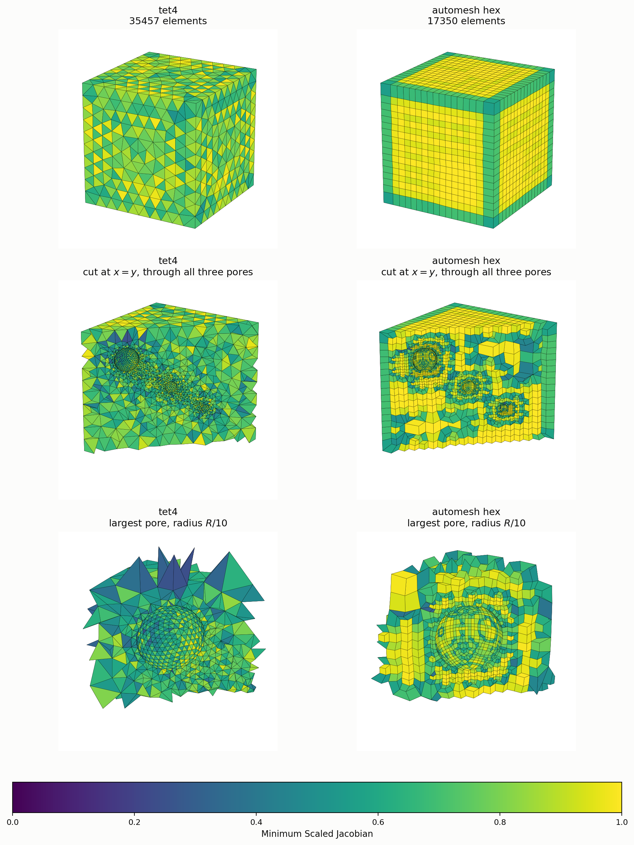
Figure 5.1.2-3: The tet4 and automesh hex meshes, painted by Minimum Scaled Jacobian
on a fixed 0 to 1 scale, so the two are comparable by color. Top row: each
mesh whole, seen from outside. Middle row: each mesh cut at the plane
. The three pore centers are collinear and all lie on that plane, so
one cut passes through every pore. Bottom row: that same cut, zoomed on the
largest pore, radius R/10. The middle and bottom rows share a camera facing
the cut plane.
Elements are kept or dropped whole, by centroid, which is what leaves the
ragged fringe around the zoomed panels. The hex mesh refines toward the pores
and holds near 1.0 through the bulk. The figure is produced by
rve_mesh_figure.py, following the style of the
autotwin/quality mesh renders.
automesh computes the same four quality measures for both meshes:
automesh metrics -i tetrahedra_4.exo -o tet4_metrics.csv
automesh metrics -i hexahedra.exo -o hex_metrics.csv
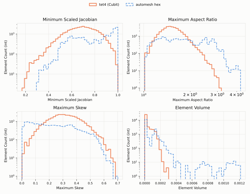
Figure 5.1.2-4: Element quality for the tet4 mesh (solid) and the automesh hex mesh
(dashed). Minimum Scaled Jacobian top left, Maximum Aspect Ratio top right,
Maximum Skew bottom left, Element Volume bottom right. Counts use a log scale.
The figure is produced by
rve_quality_histograms.py, which follows the
style of the autotwin/quality
histograms.
The hex mesh concentrates near the ideal on two of the four measures. Its scaled Jacobian piles up at 1.0, and its skew piles up at 0.0, whereas the tet4 mesh peaks near 0.45 and 0.30, respectively. The tet4 mesh holds the tighter aspect ratio, topping out near 3 while the hex mesh reaches about 4.5. Element volume separates the two most clearly. The hex mesh carries a long tail of larger elements, which is the adaptive coarsening away from the pores.
References
Cubit
Cubit builds the geometry and both tetrahedral
meshes. The journal below reproduces comparison.stl, tetrahedra_4.exo, and
tetrahedra_10.exo offered in Downloads.
#!cubit
reset

#{ R = 1 }
#{ R1 = R / 10 }
#{ R2 = R / 20 }
#{ R3 = R / 30 }
#{ THICKNESS = 10 }

create brick x 1 y 1 z 1
create sphere radius { R1 }
move volume 2 location {-1/4} {-1/4} {1/4}
create sphere radius {R2}
create sphere radius {R3}
move volume 4 location {1/5} {1/5} {-1/5}
subtract volume 2 from volume 1
subtract volume 3 from volume 5
subtract volume 4 from volume 6
export stl "comparison.stl" fast overwrite

block 1 add volume all
volume all scheme tetmesh
surface 1 2 3 4 5 6 size { 1 / THICKNESS }
surface 10 11 12 size { R / 60 }
mesh volume all
export mesh "tetrahedra_4.exo" overwrite
block 1 element type tetra10
export mesh "tetrahedra_10.exo" overwrite
Downloads
The files below are served from OneDrive/automesh/data/RVE. The first three
come from Cubit and are the inputs to this example. The last three are
produced by automesh from those inputs, using the commands on this page, and
are offered so a reader can skip straight to the results. Each checksum
below shows the first 12 hex characters of the sha256.
| file | description | size | sha256 |
|---|---|---|---|
comparison.stl | the RVE surface, exported from Cubit; input to automesh | 813 kB | 8c1861b52db7... |
tetrahedra_4.exo | the tet4 comparison mesh | 1.0 MB | b2a27385c1e8... |
tetrahedra_10.exo | the tet10 comparison mesh | 3.0 MB | f468182d956c... |
hexahedra.exo | the automesh all-hexahedral mesh | 565 kB | feeefefbebc7... |
tet4_metrics.csv | tet4 element quality, one row per element | 1.6 MB | 00854a8a695d... |
hex_metrics.csv | hex element quality, one row per element | 796 kB | ef4f509b64f1... |
Bone
The bone is a closed surface of 12,088 triangles. A long, slender shaft joins a pair of rounded lobes at each end. The model comes from the hybrid-octree meshing work of Tong, Halilaj, and Zhang [1], which meshes it with all-hexahedral elements.
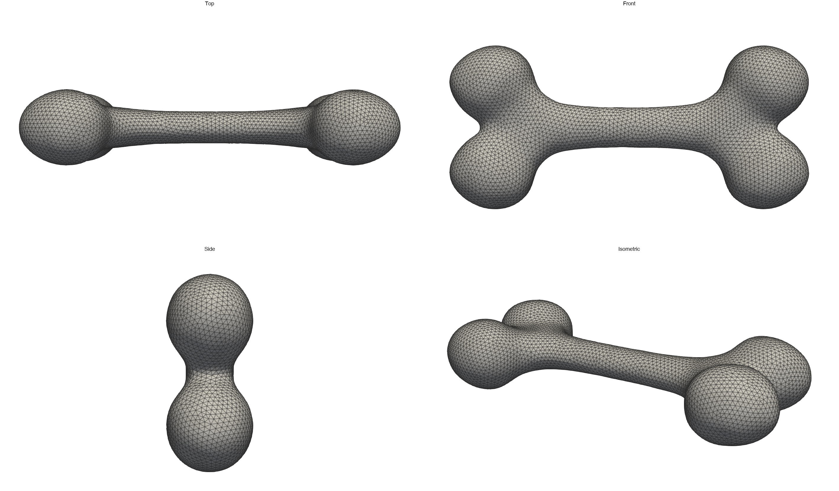
Figure 5.1.3-1: The bone surface, 12,088 triangles, in the top, front, side, and
isometric views. The triangles are close to uniform. The longest edge is
about twice the shortest. ParaView 5.10.1 makes the renders from
bone_tri_cleaned.stl (see Downloads). They come from
bone_render.py, and
bone_render_quad.py composes them.
The Tong 2024 is the baseline in this book. This page records the baseline: the settings that
produced it, its size, and its element quality. Then it meshes the same
surface with automesh and compares the two. The
Tong 2024 review
describes the method.
The method refines an octree by surface curvature and by wall thickness. It turns the octree into hexahedra, then projects the boundary onto the surface. The code rescales each model so that its longest side spans 100 units. All lengths and volumes below use that scale.
The Baseline Settings
The code, HybridOctree_Hex v1.0 [1], ships with the settings
below. Four are constants in Initialization.h: C_THRES, H_THRES,
CELL_DETECT, and VOXEL_SIZE. The curvature formula and the level of the
deepest rung are fixed inside HexGen.cpp. The published mesh comes from these
settings, as
Reproducing the Baseline shows.
| setting | value | what it sets |
|---|---|---|
| curvature formula | , summed over the edges at a vertex; fixed in the code | how sharply the surface bends at a vertex |
C_THRES | {0.15, 0.3, 0.6, 1.2, 2.4} | the curvature ladder |
H_THRES | {16, 8, 4, 2, 1} | the thickness ladder |
CELL_DETECT | 1 | which cells a vertex or triangle can split |
VOXEL_SIZE | 9 | the depth budget of the octree |
LADDER_TOP | 8 | the octree level of the deepest rung; fixed in the code |
Curvature. At each surface vertex, the code looks at every edge that meets the vertex. Two triangles share each edge. The angle between them equals on a flat surface. The code squares the deviation and sums it over the edges. The sum has units of radians squared, and nothing normalizes it. A vertex with many small triangles around it therefore gathers more terms than one with a few large triangles.
C_THRES. This is the curvature ladder. It has five rungs in ascending
order. Each rung guards one octree level. A cell at that level splits when a
vertex inside it carries a curvature above the rung.
H_THRES. This is the thickness ladder, over the same five levels. Its
rungs descend. The code measures the thickness at each triangle. It casts a
ray from the triangle's centroid along its normal, and takes the distance to
the opposite surface. A cell splits when a triangle inside it is thinner than
the rung. A cell splits when either ladder says so.
CELL_DETECT. This is a search half-width, measured in cell widths from
each cell's center. The value 1 tests a box twice the linear extent of the
cell. A vertex or triangle up to half a cell outside the cell still splits
it. A larger value refines more.
VOXEL_SIZE and LADDER_TOP. VOXEL_SIZE is the base-2 logarithm of the
octree's depth budget. The value 9 allows a grid, whose finest cells
are wide. LADDER_TOP is our name for the level of the
deepest rung. The code does not name it. It fixes the value in a test,
level == 8, inside ComputeCellValue. The value 8 puts the five rungs on
levels 4 through 8. The deepest rung
guards the step from level 8 to level 9, which is the last the budget allows.
Every level-3 cell that meets the surface splits, with no rung at all.
The Reference Mesh
| quantity | value |
|---|---|
| nodes | 10,356 |
| elements (all hexahedra) | 8,619 |
| minimum scaled Jacobian | 0.6100001 |
| total volume | 28,395.1 |
The paper publishes the mesh as bone.vtk. The file bone.inp holds the same
mesh in Abaqus format, as C3D8 elements. The nodes and elements have the
same coordinates, connectivity, and order in both files. automesh reads the
.inp file, so it computes the metrics from that one. See
Downloads for both files.
Reproducing the Baseline
We ran the code ourselves, and did not rely on the published mesh alone. The
run used HybridOctree_Hex v1.0, which is commit 00e0e82 of 2024-01-16. The
commit renames the folder HybridOctree_Hex_v1.0 to HybridOctree_Hex, and its
settings match the table above. Later commits change them. The current main
is a later version, with a VOXEL_SIZE of 10 and a different C_THRES.
The code comes from the fork
hovey/HybridOctree_Hex. We made
the fork from the original repository, CMU-CBML/HybridOctree_Hex, and it
keeps the full history, so the commit above is in it. The fork also hosts the
surface files that this page downloads. Use the folder HybridOctree_Hex at
that commit. On the fork's main, the folder HybridOctree_Hex_v1.0 is a
modified copy, and not the original code.
git clone --filter=blob:none --no-checkout https://github.com/hovey/HybridOctree_Hex.git
cd HybridOctree_Hex
git checkout 00e0e82
cd HybridOctree_Hex
c++ -std=c++17 -O2 -o HexGen Main.cpp HexGen.cpp Mesh.cpp
mkdir bone
cp "../input boundaries/bone_tri.raw" bone/model.raw
cd bone
../HexGen
The two options on the first line keep the download near 100 MB, where a plain clone of the fork is about 600 MB.
The program reads model.raw from the current directory. The build prints
warnings and no errors. We ran it on macOS, on an Apple M1 Pro, with Apple
clang 21.0.0.
The first stages took about 52 seconds: 35 seconds for the octree, 5 for the
dual mesh, and 12 for the interior mesh. Then the projection step began. It
moves the boundary nodes onto the surface, and it guards the quality of the
elements as it goes. It starts with a quality bar of 0.01. The first time the
mesh meets it, the bar jumps to 0.53. Each time the mesh meets the bar, it
writes finalMesh.vtk and raises the bar by 0.01. In our run the bar rose ten
times. The mesh written at the tenth step, after 293
iterations and about three minutes, met the bar of 0.61. The program then
searched for a mesh that meets 0.62, and did not find one. It does not stop on
its own here. We stopped it after nine minutes, and finalMesh.vtk had not
changed for the last six.
The script bone_baseline_compare.py compares that
file with the published mesh.
| published | reproduced | |
|---|---|---|
| nodes | 10,356 | 10,356 |
| elements | 8,619 | 8,619 |
| same elements, in the same order | yes | |
| minimum scaled Jacobian | 0.6100001 | 0.610002 |
| 5th percentile | 0.6103 | 0.6102 |
| median | 0.7910 | 0.7909 |
| maximum aspect ratio | 21.25 | 23.04 |
| elements above ratio 10 | 34 | 40 |
| maximum skew | 0.7252 | 0.7211 |
| maximum element volume | 39.64 | 39.65 |
The two meshes have the same nodes and the same elements, with the same connectivity, in the same order. The octree and the dual mesh reproduce exactly. Other settings would give a different octree, and so different connectivity. The floor of 0.61 reproduces, and the median and the 5th percentile agree to three digits.
The node positions do not match exactly. None of the 3,202 boundary nodes matches to six digits. They differ by 0.031 on average, and by 0.92 at most, in the units of the 100-unit cube. Of the 7,154 interior nodes, 1,563 match to six digits, and the largest difference is 1.21. The aspect ratio has a few more outliers than the published mesh.
We think the reason is the random step in the projection. The code calls
rand() and never seeds it. The generator differs between platforms. For
example, RAND_MAX is 2,147,483,647 on macOS, and the compiler warns about it.
We did not test this. We reproduced the octree, the connectivity, the quality
floor, and the shape of the quality distribution. We did not reproduce the
exact position of every node.
Minimum Scaled Jacobian
automesh computes the quality of every element:
automesh metrics -i bone.inp -o bone_reference_metrics.csv
The CSV has one row per element, in the order of the mesh. ParaView paints the elements by the Minimum Scaled Jacobian column.
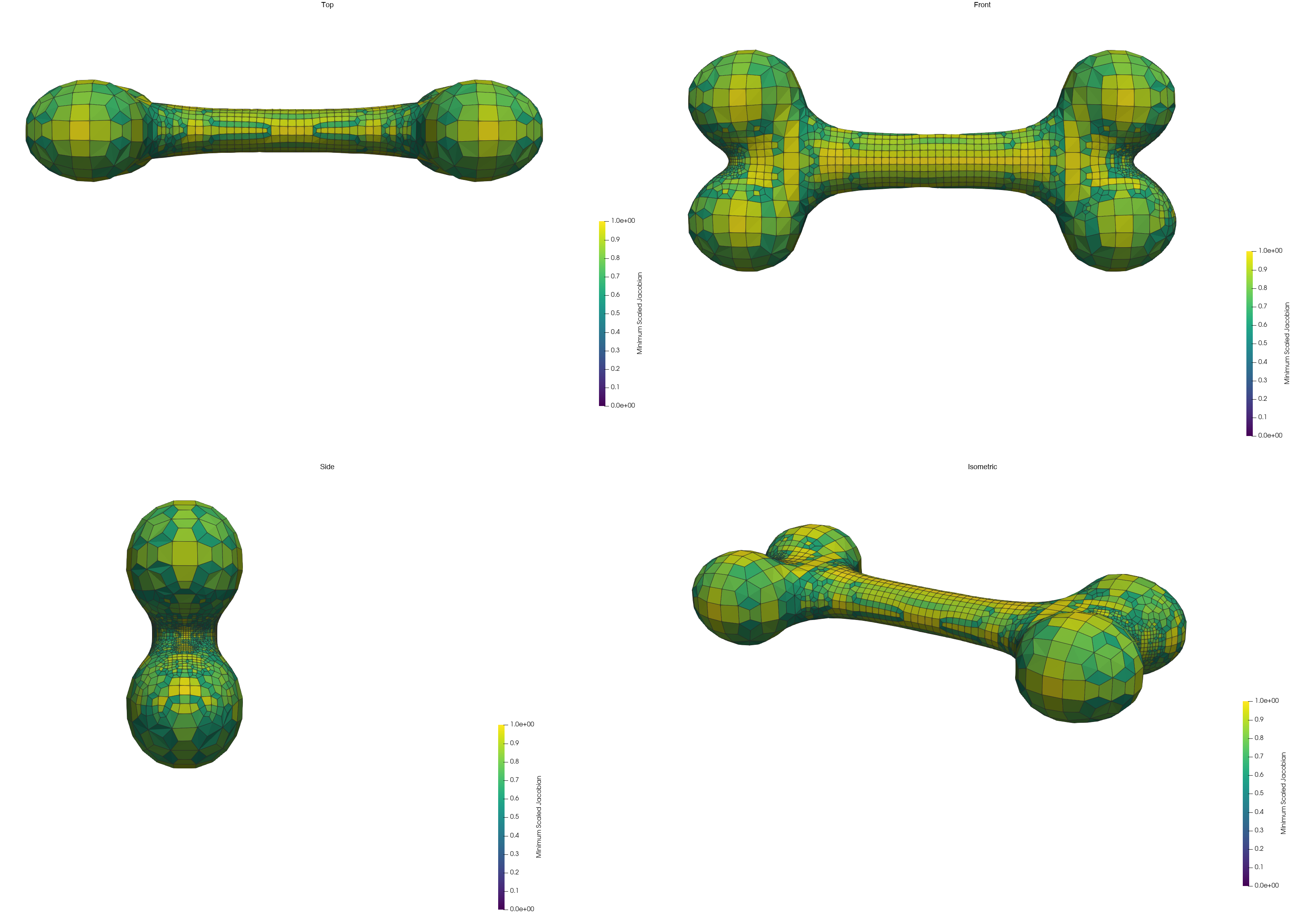
Figure 5.1.3-2: The reference bone mesh from the Tong 2024 baseline, painted by Minimum
Scaled Jacobian on a fixed 0 to 1 scale. The four panels show the top, front,
side, and isometric views. The mesh's own values run from 0.61 to 1.0, so no
element reaches the dark end of the scale. The elements are smallest on the
shaft and at the necks where the shaft meets each lobe. The lobes stay coarse.
ParaView 5.10.1 makes the renders. They come from
bone_render.py, and
bone_render_quad.py composes them.
Quality Metrics
automesh computes four measures for each element: Minimum Scaled Jacobian,
Maximum Aspect Ratio, Maximum Skew, and Element Volume [3].
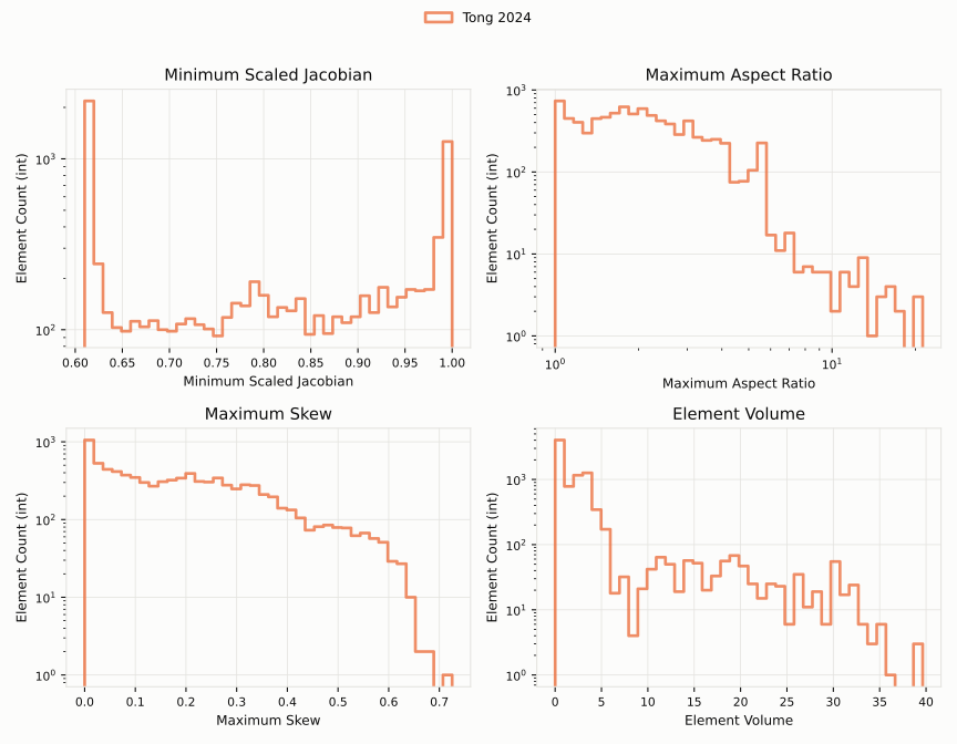
Figure 5.1.3-3: Element quality for the reference bone mesh, all 8,619 elements.
Minimum Scaled Jacobian is at top left, Maximum Aspect Ratio at top right,
Maximum Skew at bottom left, and Element Volume at bottom right. Counts use a
log scale, and the aspect ratio uses a log axis as well. The figure comes from
bone_quality_histograms.py, which follows the
style of the RVE histograms.
| measure | extreme | value |
|---|---|---|
| Minimum Scaled Jacobian | minimum | 0.6100001 |
| Maximum Aspect Ratio | maximum | 21.25 |
| Maximum Aspect Ratio | elements above 10 | 34 |
| Maximum Skew | maximum | 0.7252 |
| Element Volume | maximum | 39.64 |
The paper's title promises Jacobian control, and the mesh shows it. No element falls below a scaled Jacobian of 0.61. The values pile up at that floor, where 2,196 elements (about a quarter) sit at or below 0.62. They pile up again at 1.0, where 1,277 elements sit at or above 0.99. The median is 0.791.
The aspect ratio has a long tail. The median is 1.95, and 431 elements exceed 5. Only 34 exceed 10, and the worst reaches 21.25. The skew has a median of 0.178, and its 95th percentile is 0.497.
The element volumes span more than three orders of magnitude, from 0.0070 to 39.64, with a median of 1.48. The octree refines toward the shaft and the necks.
Meshing with automesh
automesh meshes the same surface, bone_tri_cleaned.stl, with two commands.
The first builds a uniform lattice. The second builds an adaptive octree.
Both put the mesh in the frame of the reference, so that lengths and volumes
compare directly. The scale and translate options do this. The scale is
, where 0.947288 is the longest side of the
bone in the units of the STL. The translation centers the bone in the
100-unit cube. The uniform spacing is in the units of the STL, and
.
automesh mesh hex -i bone_tri_cleaned.stl -o bone_uniform.vtu \
    --uniform 0.01563025 \
    --xscale 105.5645168 --yscale 105.5645168 --zscale 105.5645168 \
    --xtranslate -3.0485977 --ytranslate -2.8101274 --ztranslate -2.7887506 \
    --metrics bone_uniform_metrics.csv

automesh mesh hex -i bone_tri_cleaned.stl -o bone_octree.vtu --scale 7 \
    --xscale 105.5645168 --yscale 105.5645168 --zscale 105.5645168 \
    --xtranslate -3.0485977 --ytranslate -2.8101274 --ztranslate -2.7887506 \
    --metrics bone_octree_metrics.csv
The lattice gives 8,379 elements and 10,271 nodes in about 2 seconds. The
octree gives 9,267 elements and 11,381 nodes in about 1.5 seconds. Both are
close to the size of the reference. The --metrics option writes the
quality of every element, in the same four measures as before. These
numbers come from automesh 0.4.7.
Comparison
| Tong 2024 | automesh uniform lattice | automesh adaptive octree | |
|---|---|---|---|
| nodes | 10,356 | 10,271 | 11,381 |
| elements | 8,619 | 8,379 | 9,267 |
| minimum scaled Jacobian | 0.610 | 0.275 | 0.304 |
| 5th percentile | 0.610 | 0.644 | 0.531 |
| median | 0.791 | 0.884 | 0.809 |
| elements below 0.6 | 0 | 191 (2.3%) | 1,117 (12.1%) |
| maximum aspect ratio | 21.25 | 6.08 | 6.46 |
| elements above ratio 10 | 34 | 0 | 0 |
| maximum skew | 0.725 | 0.694 | 0.717 |
| maximum element volume | 39.64 | 6.64 | 18.96 |
| total volume | 28,395 | 29,236 | 29,235 |
The automesh meshes are valid. No element is inverted. The bulk of each
distribution is as good as the reference, or better. The median is higher.
The aspect ratio is far lower, with no element above 10. The skew is close.
The worst case is the difference. The reference has no element below 0.61. The lattice has a worst element at 0.275, and the octree at 0.304. The lattice has 191 elements below 0.6, and the octree has 1,117.
The reference is also graded, where the lattice is not. Its element volumes reach 39.64, while the lattice tops out at 6.64. The octree grades, and reaches 18.96.
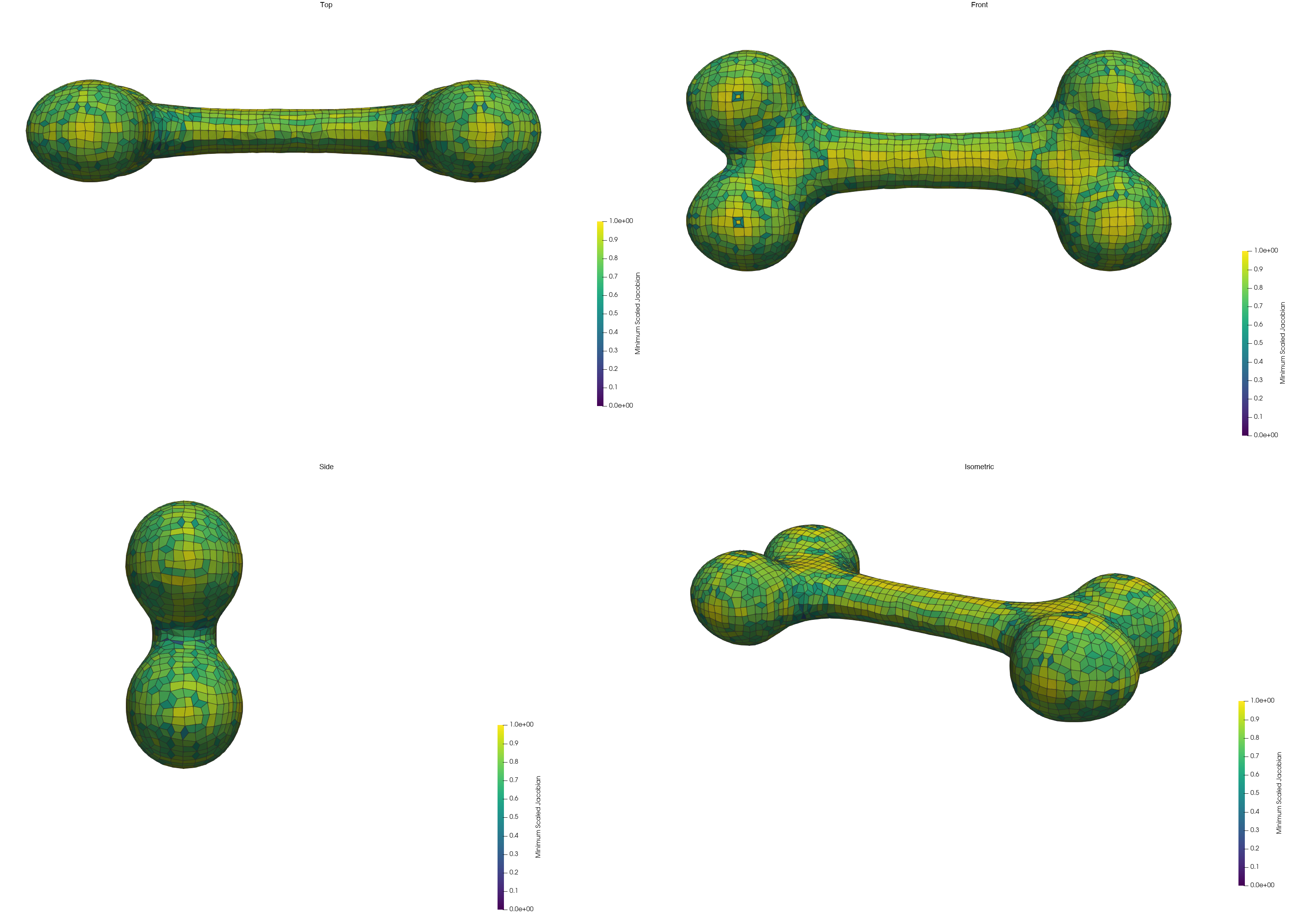
Figure 5.1.3-4: The automesh uniform-lattice mesh, painted by Minimum Scaled Jacobian
on the same 0 to 1 scale and in the same four views as the reference. The
elements are close to one size over the whole bone. A few dark elements, with
values as low as 0.28, sit scattered over the surface. The figure comes
from bone_render.py, and
bone_render_quad.py composes it.
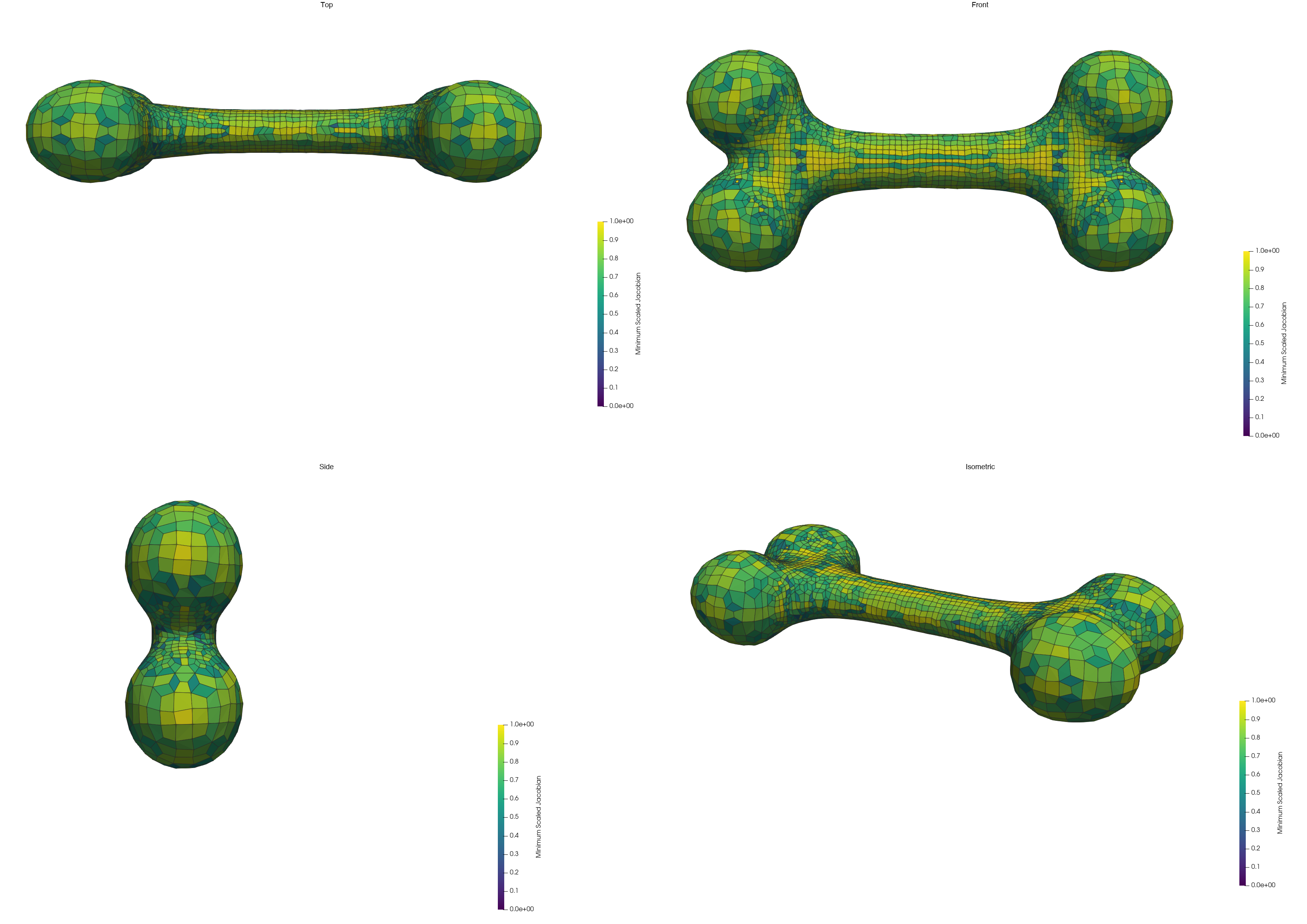
Figure 5.1.3-5: The automesh adaptive-octree mesh, painted by Minimum Scaled Jacobian
on the same scale and in the same four views. Unlike the lattice, the octree
grades. The elements are fine on the shaft and at the necks, and coarse on the
lobes, as in the reference. Several dark elements sit at the necks, where the
element size changes. The view shows only the boundary. Of the 1,117
elements below 0.6, 606 are interior, and they do not appear here. The cut
view in the next section shows them. The figure comes from the same two
scripts.
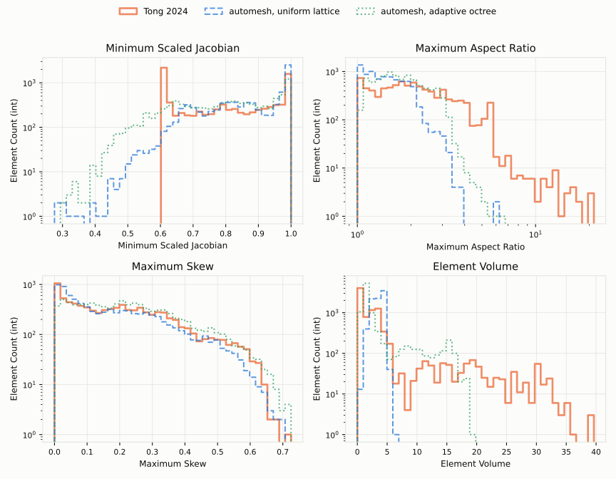
Figure 5.1.3-6: Element quality for the reference (solid, orange), the automesh
uniform lattice (dashed, blue), and the automesh adaptive octree (dotted,
green). The panels match the earlier figure. The reference has a hard floor
at 0.61 in Minimum Scaled Jacobian, and the automesh curves have a tail
toward 0.3. The lattice's tail is thin, and the octree's is fatter. The
automesh aspect ratios stay below about 6.5, where the reference reaches 21.
The figure comes from
bone_quality_histograms.py.
Where the Low Elements Are
A hex face that only one element uses lies on the boundary. The script
bone_tail.py splits the elements of each mesh into those
that touch the boundary and those that do not. In all three meshes, every
element that touches the boundary has exactly one boundary face.
| boundary elements | interior median | interior worst | boundary median | boundary worst | |
|---|---|---|---|---|---|
| Tong 2024 | 37.1% | 0.809 | 0.610 | 0.773 | 0.610 |
automesh uniform lattice | 41.6% | 0.983 | 0.575 | 0.795 | 0.275 |
automesh adaptive octree | 42.5% | 0.858 | 0.388 | 0.768 | 0.304 |
On the lattice, the interior is nearly ideal, with a median of 0.983. Of the 191 elements below 0.6, 185 (97%) touch the boundary. All 34 elements below 0.5 do. The low elements are a boundary-fit problem.
On the octree, the tail has a second source. Of the 1,117 elements below 0.6, 511 touch the boundary, and 606 are interior. The transition elements in the interior add poor elements of their own.
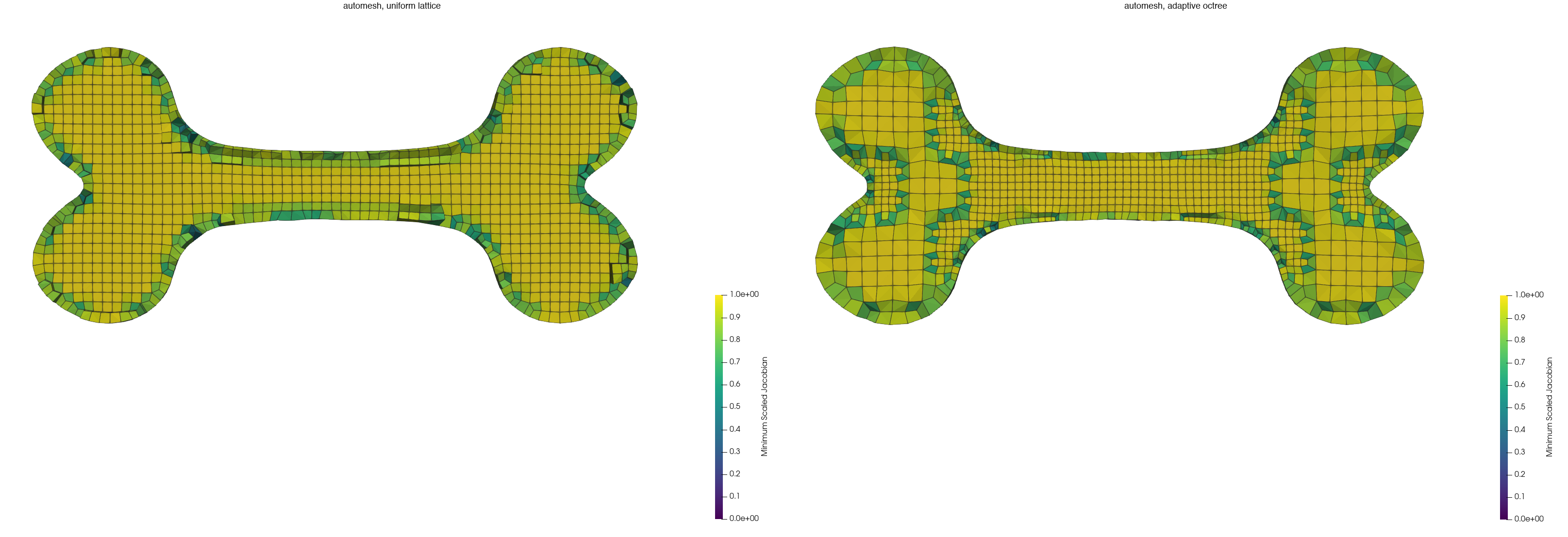
Figure 5.1.3-7: A cut through the middle of the bone, at , for the
automesh uniform lattice (left) and adaptive octree (right). Both use the
same 0 to 1 scale. An element that crosses the plane stays whole, so the cut
edge is ragged. On the lattice, the interior is a regular grid of elements
near 1.0. The low values form a thin ring at the boundary, with a few dark
elements in it. On the octree, the interior grades from coarse elements in the
lobes to fine elements in the shaft. The transitions at the necks hold teal
and green elements, and the boundary has a ring of low values as well. The
figure comes from bone_render.py with --cut, and
bone_render_quad.py composes it.
A typical boundary element is fine. The boundary median is about the same as the reference's. Only the worst boundary elements are poor. The reference holds its floor of 0.61 in both the boundary and the interior. That is consistent with a fit that guards the quality of each element. We have not confirmed this in the code of the paper.
What Did Not Help
The script bone_sweep.py runs 56 configurations of
automesh mesh hex on the bone. All 56 runs finished, and none failed. The
whole sweep took under two minutes, about 1 minute and 48 seconds, with four
runs in parallel. No configuration without smoothing raises the worst element
above 0.31.
| lever | runs | result |
|---|---|---|
| octree scale, 4 to 10 | 6 | worst element 0.19 to 0.30, with 10% to 13% of elements below 0.6 |
| weak or strong balancing, soft or snapped fit | 4 | worst element 0.298 to 0.305 |
| curvature tolerance | 15 | 4,413 to 181,175 elements, and the worst element still 0.19 to 0.30 |
| uniform spacing, 1.2 to 2.2 | 11 | worst element 0.16 to 0.29, with 1.5% to 5.2% of elements below 0.6 |
| smoothing, lattice case | 10 | worst element up to 0.36, but 3.8% to 12.7% of elements fall below 0.6, and the volume changes by 1% to 49% |
| smoothing, octree case | 10 | worst element falls to 0.14 or below, five runs invert an element, and the volume changes by 1% to 54% |
The worst element rests on a handful of boundary elements, so it is noisy. On the lattice it moves between 0.16 and 0.29 as the spacing changes. The count below 0.6 is steadier.
Smoothing does not close the gap. It moves boundary nodes off the surface, which is why the volume shrinks. On the lattice, a few iterations lift the worst element, but they raise the number of elements below 0.6.
The commands for all 56 runs
Run them from a directory that holds bone_tri_cleaned.stl. The frame options
are the same for every run, so they sit in an array. The array works in bash
and in zsh. The distances --uniform and --tolerance are in the units of
the STL, which are 105.5645168 times smaller than the frame of the reference.
bone_sweep.py converts them from the frame.
FRAME=(--xscale 105.5645168 --yscale 105.5645168 --zscale 105.5645168
       --xtranslate -3.0485977 --ytranslate -2.8101274 --ztranslate -2.7887506)

#  1. octree: scale 4
automesh mesh hex -i bone_tri_cleaned.stl -o run01.vtu --scale 4 "${FRAME[@]}" --metrics run01.csv
#  2. octree: scale 5
automesh mesh hex -i bone_tri_cleaned.stl -o run02.vtu --scale 5 "${FRAME[@]}" --metrics run02.csv
#  3. octree: scale 6
automesh mesh hex -i bone_tri_cleaned.stl -o run03.vtu --scale 6 "${FRAME[@]}" --metrics run03.csv
#  4. octree: scale 7
automesh mesh hex -i bone_tri_cleaned.stl -o run04.vtu --scale 7 "${FRAME[@]}" --metrics run04.csv
#  5. octree: scale 8
automesh mesh hex -i bone_tri_cleaned.stl -o run05.vtu --scale 8 "${FRAME[@]}" --metrics run05.csv
#  6. octree: scale 10
automesh mesh hex -i bone_tri_cleaned.stl -o run06.vtu --scale 10 "${FRAME[@]}" --metrics run06.csv
#  7. balance: scale 7, soft, weak
automesh mesh hex -i bone_tri_cleaned.stl -o run07.vtu --scale 7 "${FRAME[@]}" --metrics run07.csv
#  8. balance: scale 7, soft, strong
automesh mesh hex -i bone_tri_cleaned.stl -o run08.vtu --scale 7 --strong "${FRAME[@]}" --metrics run08.csv
#  9. balance: scale 7, snap, weak
automesh mesh hex -i bone_tri_cleaned.stl -o run09.vtu --scale 7 --snap "${FRAME[@]}" --metrics run09.csv
# 10. balance: scale 7, snap, strong
automesh mesh hex -i bone_tri_cleaned.stl -o run10.vtu --scale 7 --snap --strong "${FRAME[@]}" --metrics run10.csv
# 11. tolerance: scale 5, tolerance 1
automesh mesh hex -i bone_tri_cleaned.stl -o run11.vtu --scale 5 --tolerance 0.00947288 "${FRAME[@]}" --metrics run11.csv
# 12. tolerance: scale 5, tolerance 0.3
automesh mesh hex -i bone_tri_cleaned.stl -o run12.vtu --scale 5 --tolerance 0.00284186 "${FRAME[@]}" --metrics run12.csv
# 13. tolerance: scale 5, tolerance 0.1
automesh mesh hex -i bone_tri_cleaned.stl -o run13.vtu --scale 5 --tolerance 0.00094729 "${FRAME[@]}" --metrics run13.csv
# 14. tolerance: scale 5, tolerance 0.03
automesh mesh hex -i bone_tri_cleaned.stl -o run14.vtu --scale 5 --tolerance 0.00028419 "${FRAME[@]}" --metrics run14.csv
# 15. tolerance: scale 5, tolerance 0.01
automesh mesh hex -i bone_tri_cleaned.stl -o run15.vtu --scale 5 --tolerance 0.00009473 "${FRAME[@]}" --metrics run15.csv
# 16. tolerance: scale 6, tolerance 1
automesh mesh hex -i bone_tri_cleaned.stl -o run16.vtu --scale 6 --tolerance 0.00947288 "${FRAME[@]}" --metrics run16.csv
# 17. tolerance: scale 6, tolerance 0.3
automesh mesh hex -i bone_tri_cleaned.stl -o run17.vtu --scale 6 --tolerance 0.00284186 "${FRAME[@]}" --metrics run17.csv
# 18. tolerance: scale 6, tolerance 0.1
automesh mesh hex -i bone_tri_cleaned.stl -o run18.vtu --scale 6 --tolerance 0.00094729 "${FRAME[@]}" --metrics run18.csv
# 19. tolerance: scale 6, tolerance 0.03
automesh mesh hex -i bone_tri_cleaned.stl -o run19.vtu --scale 6 --tolerance 0.00028419 "${FRAME[@]}" --metrics run19.csv
# 20. tolerance: scale 6, tolerance 0.01
automesh mesh hex -i bone_tri_cleaned.stl -o run20.vtu --scale 6 --tolerance 0.00009473 "${FRAME[@]}" --metrics run20.csv
# 21. tolerance: scale 7, tolerance 1
automesh mesh hex -i bone_tri_cleaned.stl -o run21.vtu --scale 7 --tolerance 0.00947288 "${FRAME[@]}" --metrics run21.csv
# 22. tolerance: scale 7, tolerance 0.3
automesh mesh hex -i bone_tri_cleaned.stl -o run22.vtu --scale 7 --tolerance 0.00284186 "${FRAME[@]}" --metrics run22.csv
# 23. tolerance: scale 7, tolerance 0.1
automesh mesh hex -i bone_tri_cleaned.stl -o run23.vtu --scale 7 --tolerance 0.00094729 "${FRAME[@]}" --metrics run23.csv
# 24. tolerance: scale 7, tolerance 0.03
automesh mesh hex -i bone_tri_cleaned.stl -o run24.vtu --scale 7 --tolerance 0.00028419 "${FRAME[@]}" --metrics run24.csv
# 25. tolerance: scale 7, tolerance 0.01
automesh mesh hex -i bone_tri_cleaned.stl -o run25.vtu --scale 7 --tolerance 0.00009473 "${FRAME[@]}" --metrics run25.csv
# 26. uniform: spacing 1.2
automesh mesh hex -i bone_tri_cleaned.stl -o run26.vtu --uniform 0.01136746 "${FRAME[@]}" --metrics run26.csv
# 27. uniform: spacing 1.3
automesh mesh hex -i bone_tri_cleaned.stl -o run27.vtu --uniform 0.01231474 "${FRAME[@]}" --metrics run27.csv
# 28. uniform: spacing 1.4
automesh mesh hex -i bone_tri_cleaned.stl -o run28.vtu --uniform 0.01326203 "${FRAME[@]}" --metrics run28.csv
# 29. uniform: spacing 1.5
automesh mesh hex -i bone_tri_cleaned.stl -o run29.vtu --uniform 0.01420932 "${FRAME[@]}" --metrics run29.csv
# 30. uniform: spacing 1.6
automesh mesh hex -i bone_tri_cleaned.stl -o run30.vtu --uniform 0.01515661 "${FRAME[@]}" --metrics run30.csv
# 31. uniform: spacing 1.65
automesh mesh hex -i bone_tri_cleaned.stl -o run31.vtu --uniform 0.01563025 "${FRAME[@]}" --metrics run31.csv
# 32. uniform: spacing 1.7
automesh mesh hex -i bone_tri_cleaned.stl -o run32.vtu --uniform 0.01610390 "${FRAME[@]}" --metrics run32.csv
# 33. uniform: spacing 1.8
automesh mesh hex -i bone_tri_cleaned.stl -o run33.vtu --uniform 0.01705118 "${FRAME[@]}" --metrics run33.csv
# 34. uniform: spacing 1.9
automesh mesh hex -i bone_tri_cleaned.stl -o run34.vtu --uniform 0.01799847 "${FRAME[@]}" --metrics run34.csv
# 35. uniform: spacing 2.0
automesh mesh hex -i bone_tri_cleaned.stl -o run35.vtu --uniform 0.01894576 "${FRAME[@]}" --metrics run35.csv
# 36. uniform: spacing 2.2
automesh mesh hex -i bone_tri_cleaned.stl -o run36.vtu --uniform 0.02084034 "${FRAME[@]}" --metrics run36.csv
# 37. smooth: uniform 1.65, Taubin 5
automesh mesh hex -i bone_tri_cleaned.stl -o run37.vtu --uniform 0.01563025 "${FRAME[@]}" --metrics run37.csv smooth -m Taubin -n 5
# 38. smooth: uniform 1.65, Taubin 5, hierarchical
automesh mesh hex -i bone_tri_cleaned.stl -o run38.vtu --uniform 0.01563025 "${FRAME[@]}" --metrics run38.csv smooth -m Taubin -n 5 --hierarchical
# 39. smooth: uniform 1.65, Taubin 20
automesh mesh hex -i bone_tri_cleaned.stl -o run39.vtu --uniform 0.01563025 "${FRAME[@]}" --metrics run39.csv smooth -m Taubin -n 20
# 40. smooth: uniform 1.65, Taubin 20, hierarchical
automesh mesh hex -i bone_tri_cleaned.stl -o run40.vtu --uniform 0.01563025 "${FRAME[@]}" --metrics run40.csv smooth -m Taubin -n 20 --hierarchical
# 41. smooth: uniform 1.65, Taubin 50
automesh mesh hex -i bone_tri_cleaned.stl -o run41.vtu --uniform 0.01563025 "${FRAME[@]}" --metrics run41.csv smooth -m Taubin -n 50
# 42. smooth: uniform 1.65, Taubin 50, hierarchical
automesh mesh hex -i bone_tri_cleaned.stl -o run42.vtu --uniform 0.01563025 "${FRAME[@]}" --metrics run42.csv smooth -m Taubin -n 50 --hierarchical
# 43. smooth: uniform 1.65, Taubin 100
automesh mesh hex -i bone_tri_cleaned.stl -o run43.vtu --uniform 0.01563025 "${FRAME[@]}" --metrics run43.csv smooth -m Taubin -n 100
# 44. smooth: uniform 1.65, Taubin 100, hierarchical
automesh mesh hex -i bone_tri_cleaned.stl -o run44.vtu --uniform 0.01563025 "${FRAME[@]}" --metrics run44.csv smooth -m Taubin -n 100 --hierarchical
# 45. smooth: uniform 1.65, Laplace 5
automesh mesh hex -i bone_tri_cleaned.stl -o run45.vtu --uniform 0.01563025 "${FRAME[@]}" --metrics run45.csv smooth -m Laplace -n 5
# 46. smooth: uniform 1.65, Laplace 20
automesh mesh hex -i bone_tri_cleaned.stl -o run46.vtu --uniform 0.01563025 "${FRAME[@]}" --metrics run46.csv smooth -m Laplace -n 20
# 47. smooth: scale 7, Taubin 5
automesh mesh hex -i bone_tri_cleaned.stl -o run47.vtu --scale 7 "${FRAME[@]}" --metrics run47.csv smooth -m Taubin -n 5
# 48. smooth: scale 7, Taubin 5, hierarchical
automesh mesh hex -i bone_tri_cleaned.stl -o run48.vtu --scale 7 "${FRAME[@]}" --metrics run48.csv smooth -m Taubin -n 5 --hierarchical
# 49. smooth: scale 7, Taubin 20
automesh mesh hex -i bone_tri_cleaned.stl -o run49.vtu --scale 7 "${FRAME[@]}" --metrics run49.csv smooth -m Taubin -n 20
# 50. smooth: scale 7, Taubin 20, hierarchical
automesh mesh hex -i bone_tri_cleaned.stl -o run50.vtu --scale 7 "${FRAME[@]}" --metrics run50.csv smooth -m Taubin -n 20 --hierarchical
# 51. smooth: scale 7, Taubin 50
automesh mesh hex -i bone_tri_cleaned.stl -o run51.vtu --scale 7 "${FRAME[@]}" --metrics run51.csv smooth -m Taubin -n 50
# 52. smooth: scale 7, Taubin 50, hierarchical
automesh mesh hex -i bone_tri_cleaned.stl -o run52.vtu --scale 7 "${FRAME[@]}" --metrics run52.csv smooth -m Taubin -n 50 --hierarchical
# 53. smooth: scale 7, Taubin 100
automesh mesh hex -i bone_tri_cleaned.stl -o run53.vtu --scale 7 "${FRAME[@]}" --metrics run53.csv smooth -m Taubin -n 100
# 54. smooth: scale 7, Taubin 100, hierarchical
automesh mesh hex -i bone_tri_cleaned.stl -o run54.vtu --scale 7 "${FRAME[@]}" --metrics run54.csv smooth -m Taubin -n 100 --hierarchical
# 55. smooth: scale 7, Laplace 5
automesh mesh hex -i bone_tri_cleaned.stl -o run55.vtu --scale 7 "${FRAME[@]}" --metrics run55.csv smooth -m Laplace -n 5
# 56. smooth: scale 7, Laplace 20
automesh mesh hex -i bone_tri_cleaned.stl -o run56.vtu --scale 7 "${FRAME[@]}" --metrics run56.csv smooth -m Laplace -n 20
What This Means
automesh matches the bulk of the reference and beats it on aspect ratio. It
does not match the worst case. The minimum scaled Jacobian is near 0.3, where
the reference holds 0.61. The gap sits in the elements on the boundary.
What the study shows. None of the levers that set the size, the scale, the balancing, the fit, the tolerance, or the spacing raises the worst element above about 0.31. Smoothing lifts it to 0.36 at most. It also costs volume and raises the count of elements below 0.6. These levers change how many elements the mesh has. They do not change how bad the worst boundary elements are. For this bone, the result is solid.
What it does not show. The study does not show that one method is the answer. It shows what does not work, where the low elements sit, and how the reference works. The reference method is a ratchet. Its code raises a quality bar in steps of 0.01, up to 0.61 in our run. It moves a boundary node only when the neighboring elements stay above the bar. The hard floor of the reference is that bar.
The study did not try the alternatives. Better initial fitting is one, and
issue autotwin/automesh#750
holds the results of Protais, Cherchi, and Livesu. The smooth fit oracle in
conspire PR #186 is
another. Local topology repair of the worst elements is a third. Any of them
could raise the floor without being a ratchet. A quality guard is the one
approach we know of that gives a floor by construction. Better fitting improves
the distribution, but it cannot promise a floor.
Two guards may be needed. On the lattice, 97% of the elements below 0.6 touch the boundary, so a guard on the boundary fit targets them. On the octree, about half of the tail is interior transition elements: 606 of 1,117. A guard on the boundary alone would leave them. The interior needs the same guard, or better transition templates.
The smallest version. A guarded smoother is the smallest step toward a
ratchet. It moves a node toward a better position. It accepts the move only if
no neighboring element drops below the current bar. Then it raises the bar and
repeats. The smoothing of automesh has no guard today. That is why it
inverts elements and shrinks the volume. A guard, together with keeping the
boundary nodes on the surface, would fix both faults.
A test we have not run. A prototype on the lattice mesh would show how far a guard goes. It would use the acceptance rule of the reference, and the same steps of 0.01 in the bar. It would report how high the worst element climbs, and how many elements stay below 0.6. If the floor rises toward 0.6, a guard is enough. If it stalls near 0.4, the fit needs more. The issue autotwin/automesh#768 tracks this, with the bone as the benchmark.
Reproducibility
The inputs are not committed. See Downloads to get them. From this directory:
The commands that regenerate the figures and tables follow:
PVPYTHON=/Applications/ParaView-5.10.1.app/Contents/bin/pvpython

# the surface figure
for view in top front side iso; do
    $PVPYTHON --force-offscreen-rendering bone_render.py \
        bone_tri_cleaned.stl bone_surface_$view.png --view $view
done
uv run --with pillow bone_render_quad.py bone_surface_top.png \
    bone_surface_front.png bone_surface_side.png bone_surface_iso.png \
    bone_surface.png

# the Minimum Scaled Jacobian figure
automesh metrics -i bone.inp -o bone_reference_metrics.csv
for view in top front side iso; do
    $PVPYTHON --force-offscreen-rendering bone_render.py \
        bone.vtk bone_msj_$view.png --view $view \
        --metrics bone_reference_metrics.csv
done
uv run --with pillow bone_render_quad.py bone_msj_top.png bone_msj_front.png \
    bone_msj_side.png bone_msj_iso.png bone_reference_msj.png

# the histograms of the reference
uv run --with numpy --with matplotlib bone_quality_histograms.py \
    bone_quality_histograms.svg --mesh bone_reference_metrics.csv "Tong 2024"

# the two automesh meshes: the commands in the section above, then
for view in top front side iso; do
    $PVPYTHON --force-offscreen-rendering bone_render.py \
        bone_uniform.vtu bone_uniform_$view.png --view $view \
        --metrics bone_uniform_metrics.csv
done
uv run --with pillow bone_render_quad.py bone_uniform_top.png \
    bone_uniform_front.png bone_uniform_side.png bone_uniform_iso.png \
    bone_automesh_msj.png

for view in top front side iso; do
    $PVPYTHON --force-offscreen-rendering bone_render.py \
        bone_octree.vtu bone_octree_$view.png --view $view \
        --metrics bone_octree_metrics.csv
done
uv run --with pillow bone_render_quad.py bone_octree_top.png \
    bone_octree_front.png bone_octree_side.png bone_octree_iso.png \
    bone_octree_msj.png

# a cut through both meshes, side by side
for mesh in uniform octree; do
    $PVPYTHON --force-offscreen-rendering bone_render.py \
        bone_$mesh.vtu bone_cut_$mesh.png --view front --cut \
        --metrics bone_${mesh}_metrics.csv
done
uv run --with pillow bone_render_quad.py bone_cut_uniform.png \
    bone_cut_octree.png bone_cut_msj.png --columns 2 \
    --label "automesh, uniform lattice" --label "automesh, adaptive octree"

# the overlay histograms
uv run --with numpy --with matplotlib bone_quality_histograms.py \
    bone_quality_comparison.svg \
    --mesh bone_reference_metrics.csv "Tong 2024" \
    --mesh bone_uniform_metrics.csv "automesh, uniform lattice" \
    --mesh bone_octree_metrics.csv "automesh, adaptive octree"

# where the low elements are
python3 bone_tail.py bone.inp bone_reference_metrics.csv
python3 bone_tail.py bone_uniform.vtu bone_uniform_metrics.csv
python3 bone_tail.py bone_octree.vtu bone_octree_metrics.csv

# the sweep of 56 runs, about two minutes
python3 bone_sweep.py bone_sweep.tsv

# compare the reproduced baseline with the published mesh, after the run in
# the section Reproducing the Baseline; copy its finalMesh.vtk here first
cp path/to/bone/finalMesh.vtk reproduced_bone.vtk
python3 bone_baseline_compare.py reproduced_bone.vtk bone.vtk
The histogram commands print the extremes in the tables above.
References
- Hua Tong, Eni Halilaj, and Yongjie Jessica Zhang. "HybridOctree_Hex:
Hybrid octree-based adaptive all-hexahedral mesh generation with Jacobian
control." Journal of Computational Science 78 (2024) 102278.
https://doi.org/10.1016/j.jocs.2024.102278. The code is at
https://github.com/CMU-CBML/HybridOctree_Hex. The run on this page used
commit
00e0e82. - Utkarsh Ayachit. The ParaView Guide: A Parallel Visualization Application. Kitware, 2015. https://www.paraview.org.
- Patrick M. Knupp, C. D. Ernst, D. C. Thompson, C. J. Stimpson, and P. P. Pebay. The Verdict Geometric Quality Library. SAND2007-1751, Sandia National Laboratories, 2006. https://www.osti.gov/servlets/purl/901967.
Downloads
The files below are served from the
hovey/HybridOctree_Hex
repository. Each checksum shows the first 12 hex characters of the sha256.
| file | description | size | sha256 |
|---|---|---|---|
bone.vtk | the reference mesh, as published with the paper | 690 kB | 88dd3cb24fcb... |
bone.inp | the same mesh in Abaqus format; input to automesh metrics | 840 kB | c34d184981f8... |
bone_tri.raw | the surface the code meshes, in its .raw format | 338 kB | c37284adbab5... |
bone_tri_cleaned.stl | the same 12,088 triangles as an STL; the surface in the top figure, and the file automesh reads | 604 kB | 9871e33c65c6... |
The .raw file lists one point that no triangle uses. The cleaned files drop
that point and leave the surface unchanged. The repository also holds them as
bone_tri_cleaned.raw, bone_tri_cleaned.off, and bone_tri_cleaned.obj.
Industry Models
Where Academic Models are chosen for geometric pathology, these are chosen for practical relevance: parts representative of real mechanical design and analysis work — manufactured features, assemblies, and engineering benchmarks. None are in the repository yet; sourcing is left open rather than pointing at specific unverified links.
The table below tracks candidate models and their status. All entries are currently "Planned" — a roadmap, not a claim that a model is already available.
| Model | Description | Status |
|---|---|---|
| Engine block | multi-cavity cast part; internal/external surfaces | Planned |
| Connecting rod | classic FE benchmark geometry | Planned |
| Bracket / mounting plate | sheet/machined part with holes and fillets | Planned |
| Gear | involute tooth profile; fine periodic surface detail | Planned |
| Turbine blade | thin curved aerofoil surface | Planned |
| Heat sink | dense fin array; thin-feature stress test | Planned |
| Pressure vessel | thin-shell enclosure | Planned |
Analysis
This section contains analysis that is used to answer questions pertaining to
mesh creation, quality, resolution, and convergence.
Sphere with Shells follows a single model
end to end — voxel meshing, sculpting, simulation, a conforming Cubit mesh
built for comparison, automesh smoothing, and a final comparison between
the two approaches. Conforming v Segmented Meshes
compares a conforming mesh against its segment-derived voxelized
counterpart.
Sphere with Shells
This section presents a model composed of a sphere with two concentric shells. We use the model to explore answers to the following questions:
- What compute time is required to create successively refined resolutions in
automesh? - What compute time is required to create these same resolutions in Sculpt?
- Given a rotational boundary condition, what are the displacement and strain fields for the voxel mesh?
- How do the results for the voxel mesh compare with the results for a conforming mesh?
- To what degree may smoothing the voxel mesh improve the results?
- To what degree may dualization of the voxel mesh improve the results?
Model
Python is used to create a segmentations, saved as .npy files, and visualize the results.
Given
Given three concentric spheres of radius 10, 11, and 12 cm, as shown in the figure below,
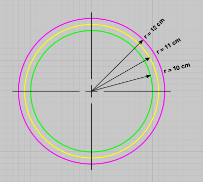
Figure 6.1-1: Schematic cross-section of three concentric spheres of radius 10, 11, and 12 cm. Grid spacing is 1 cm.
Find
Use segmentation resolutions 1, 2, 4, and 10 voxels per centimeter
with a cubic domain (nelx = nely = nelz) to create finite element meshes.
Solution
| vox/cm | element side length (cm) | nelx | # voxels | segmentation | file size |
|---|---|---|---|---|---|
| 1 | 1.0 | 24 | 13,824 | spheres_resolution_1.npy | 14 kB |
| 2 | 0.5 | 48 | 110,592 | spheres_resolution_2.npy | 111 kB |
| 4 | 0.25 | 96 | 884,736 | spheres_resolution_3.npy | 885 kB |
| 10 | 0.1 | 240 | 13,824,000 | spheres_resolution_4.npy | 13.78 MB |
Python Segmentation
The Python code used to generate the figures is included below.
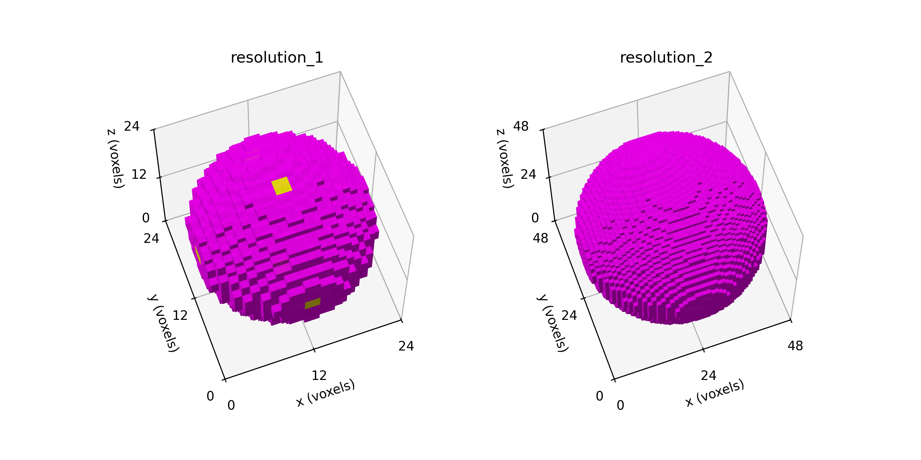
Figure 6.1-2: Sphere segmentations (left) spheres_resolution_1.npy and (right) spheres_resolution_2.npy shown in the voxel domain.
Because plotting large domains with Matplotlib
is slow, only the first two resolutions are shown.
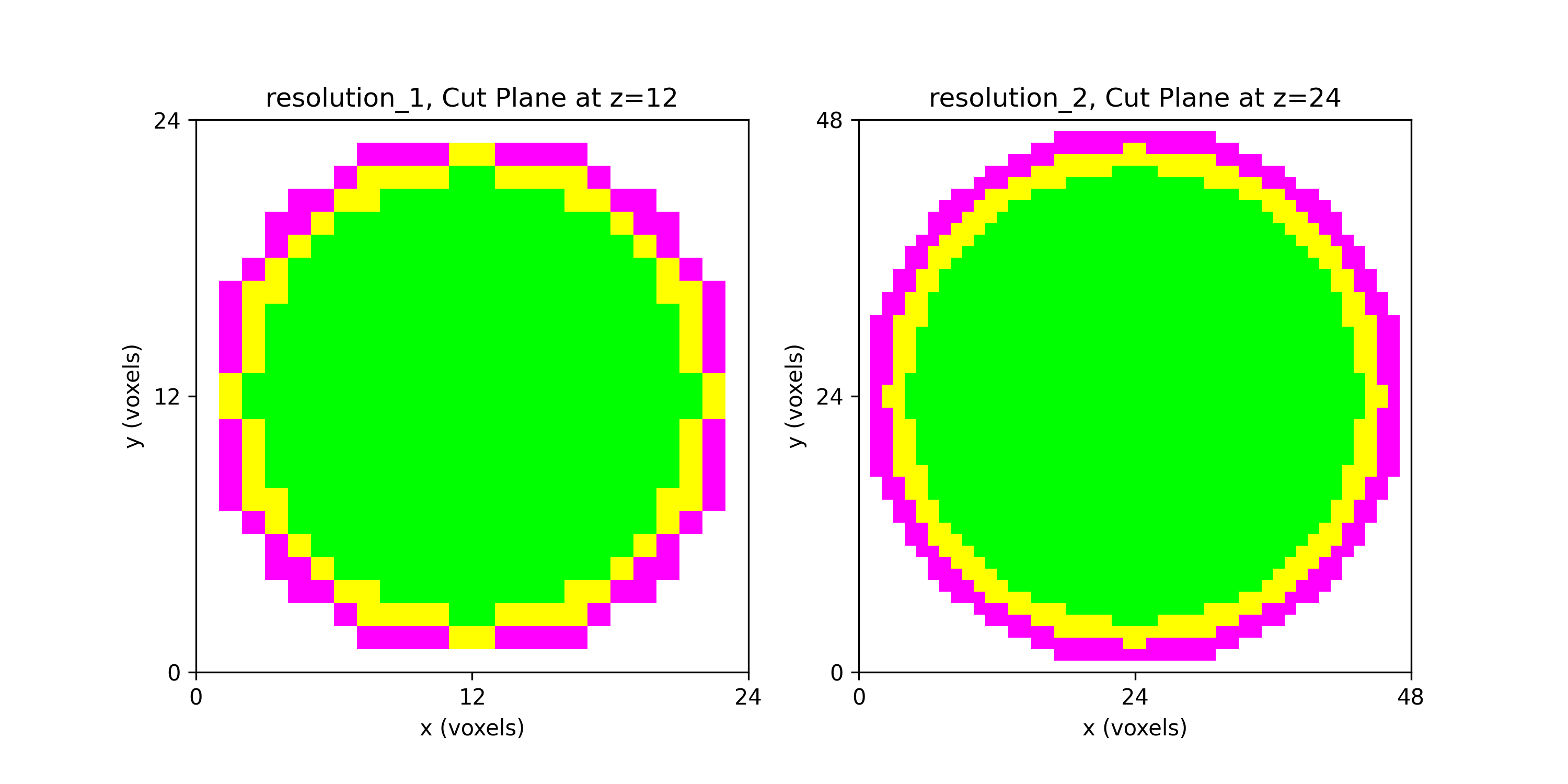
Figure 6.1-3: Sphere segmentations with cutting plane of (left) spheres_resolution_1.npy and (right) spheres_resolution_2.npy.
Source
spheres_cont.py
spheres_cont.py
r"""This module, spheres_cont.py, builds on the spheres.py module to create
high resolution, three-material, concentric spheres and export the
voxelization as a .npy file.

Example
-------
source ~/autotwin/automesh/.venv/bin/activate
python spheres_cont.py

Output
------
~/autotwin/automesh/book/analysis/sphere_with_shells/spheres_resolution_1.npy
~/autotwin/automesh/book/analysis/sphere_with_shells/spheres_resolution_2.npy
~/autotwin/automesh/book/analysis/sphere_with_shells/spheres_resolution_3.npy
~/autotwin/automesh/book/analysis/sphere_with_shells/spheres_resolution_4.npy
"""

from pathlib import Path
from typing import Final

from matplotlib.colors import LightSource, ListedColormap
import matplotlib.pyplot as plt
from mpl_toolkits.mplot3d import Axes3D
import numpy as np


# Visualize on a cutting plane
def plot_cutting_plane(ax, key, data, plane="z", index=None, cmap=None, alpha=None):
    """Plots a 2D cutting plane slice of a 3D dataset on the specified axis.

    This function visualizes a slice of the 3D data array along a specified
    plane (x, y, or z) and displays it using a 2D image representation. The
    slice can be specified by an index, and the appearance of the plot can be
    customized with a colormap and transparency level.

    Parameters
    ----------
    ax : matplotlib.axes.Axes
        The axes on which to plot the cutting plane.

    key : str
        A descriptive label for the dataset, used in the plot title.

    data : numpy.ndarray
        A 3D numpy array representing the voxelized data. The shape of the
        array should be (depth, height, width) corresponding to the
        z, y, and x dimensions.

    plane : str, optional
        The plane along which to slice the data. Can be 'x', 'y', or 'z'.
        Default is 'z'.

    index : int, optional
        The index of the slice to visualize along the specified plane. If not
        provided, the function will default to the middle slice of the data
        along the specified plane.

    cmap : str or matplotlib.colors.Colormap, optional
        The colormap to use for visualizing the slice. If not provided,
        defaults to 'gray'.

    alpha : float, optional
        The transparency level of the plotted slice, where 0 is fully
        transparent and 1 is fully opaque. If not provided, defaults to 0.8.

    Returns
    -------
    None
        This function does not return any value. It modifies the provided axes
        to display the cutting plane visualization.

    Notes
    -----
    The function sets the x and y labels based on the specified plane and
    adjusts the plot title to include the key and the index of the slice.
    """
    origin = "lower"
    if cmap is None:
        cmap = "gray"
    if alpha is None:
        alpha = 0.8
    if plane == "z":
        if index is None:
            index = data.shape[2] // 2  # Middle slice
        slice_data = data[:, :, index]
        ax.imshow(
            slice_data,
            cmap=cmap,
            extent=[0, data.shape[1], 0, data.shape[0]],
            origin=origin,
            alpha=alpha,
        )
        ax.set_title(f"{key}, Cut Plane at z={index}")
        ax.set_xlabel("x (voxels)")
        ax.set_ylabel("y (voxels)")
    elif plane == "y":
        if index is None:
            index = data.shape[1] // 2  # Middle slice
        slice_data = data[:, index, :]
        ax.imshow(
            slice_data,
            cmap=cmap,
            extent=[0, data.shape[2], 0, data.shape[0]],
            origin=origin,
            alpha=alpha,
        )
        ax.set_title(f"{key}, Cut Plane at y={index}")
        ax.set_xlabel("x (voxels)")
        ax.set_ylabel("z (voxels)")
    elif plane == "x":
        if index is None:
            index = data.shape[0] // 2  # Middle slice
        slice_data = data[index, :, :]
        ax.imshow(
            slice_data,
            cmap=cmap,
            extent=[0, data.shape[2], 0, data.shape[1]],
            origin=origin,
            alpha=alpha,
        )
        ax.set_title(f"{key} Cut Plane at x={index}")
        ax.set_xlabel("y (voxels)")
        ax.set_ylabel("z (voxels)")


def sphere(resolution: int, dtype=np.uint8) -> np.ndarray:
    """Generate a 3D voxelized representation of three concentric spheres
    of 10, 11, and 12 cm, at a given resolution.

    Parameters
    ----------
    resolution : int
        The resolution as voxels per centimeter.  Minimum value is 1.

    dtype: data-type, optional
        The data type of the output array.  Default is np.uint8.

    Returns
    -------
    np.ndarray
        A 3D numpy array representing the voxelized spheres.  Voxels within
        the inner sphere are set to 1, the intermediate shell are set to 2,
        and the outer shell are set to 3.  Voxels outside the spheres are
        set to 0.

    Raises
    ------
    ValueError
        If the resolution is less than 1.
    """
    print(f"Creating sphere with resolution: {resolution}")
    if resolution < 1:
        raise ValueError("Resolution must be >= 1")

    r10 = 10  # cm
    r11 = 11  # cm
    r12 = 12  # cm

    # We change the algorithm a bit here so we can exactly match the radius:
    # number of voxels per side length (nvps)
    # nvps = 2 * r12 * resolution + 1
    nvps = 2 * r12 * resolution
    vox_z, vox_y, vox_x = np.mgrid[
        -r12 : r12 : nvps * 1j,
        -r12 : r12 : nvps * 1j,
        -r12 : r12 : nvps * 1j,
    ]
    domain = vox_x**2 + vox_y**2 + vox_z**2

    # sphere with radius 10, indicated with "1" and background as "0"
    mask_10_in = np.array(domain <= r10 * r10, dtype=dtype)  # segmentation "1"
    # sphere with radius 11, indicated with "1" and background as "0"
    mask_11_in = np.array(domain <= r11 * r11, dtype=dtype)
    # sphere with radius 12, indicated with "1" and background as "0"
    mask_12_in = np.array(domain <= r12 * r12, dtype=dtype)

    mask_10_11 = mask_11_in - mask_10_in  # intermediate shell
    mask_11_12 = mask_12_in - mask_11_in  # outer shell

    # mask_10_in is already the inner sphere, segmentation "1"
    shell_10_11 = 2 * mask_10_11  # intermediate shell, segmentation "2"
    shell_11_12 = 3 * mask_11_12  # outer shell, segmentation "3"

    result = mask_10_in + shell_10_11 + shell_11_12
    print(f"Completed: Sphere with resolution: {resolution}")
    return result


def main():
    """The main program."""
    # rr = (1, 2, 4, 10)  # resolutions (voxels per cm)
    rr = (1, 2)  # resolutions (voxels per cm)
    lims = tuple(map(lambda x: [0, 24 * x], rr))  # limits
    tt = tuple(map(lambda x: [0, 12 * x, 24 * x], rr))  # ticks

    # User input begin
    spheres = {
        f"resolution_{i + 1}": sphere(resolution=res) for i, res in enumerate(rr)
    }

    aa = Path(__file__)

    # Visualize the elements.
    width, height = 10, 5
    # width, height = 8, 4
    # width, height = 6, 3
    fig = plt.figure(figsize=(width, height))
    fig2 = plt.figure(figsize=(width, height))

    el, az, roll = 63, -110, 0
    VOXEL_ALPHA: Final[float] = 0.9
    CUT_ALPHA: Final[float] = 1.0

    lightsource = LightSource(azdeg=325, altdeg=45)  # azimuth, elevation
    # lightsource = LightSource(azdeg=325, altdeg=90)  # azimuth, elevation
    DPI: Final[int] = 300  # resolution, dots per inch
    SHOW: Final[bool] = True  # turn to True to show the figure on screen
    SAVE: Final[bool] = True  # turn to True to save .png and .npy files

    # Define the custom colormap
    # Define the color mapping
    # 0: transparent (no color), 1: green, 2: yellow
    colors = [
        (1, 1, 1, 0),  # Transparent for segmentation "0"
        (0, 1, 0, 1),  # Green for segmentation "1"
        (1, 1, 0, 1),  # Yellow for segmentation "2"
        (1, 0, 1, 1),  # Magenta for segmentation "3"
    ]
    custom_cmap = ListedColormap(colors)
    # User input end

    N_SUBPLOTS = len(spheres)
    for index, (key, value) in enumerate(spheres.items()):
        if SHOW:
            print(f"index: {index}")
            print(f"key: {key}")
            # print(f"value: {value}")
            ax = fig.add_subplot(1, N_SUBPLOTS, index + 1, projection=Axes3D.name)
            # Create an array for face colors based on the values in the
            # `value` array
            facecolors = np.empty(
                value.shape + (4,), dtype=float
            )  # Shape (x, y, z, 4) for RGBA

            for i in range(value.shape[0]):
                for j in range(value.shape[1]):
                    for k in range(value.shape[2]):
                        facecolors[i, j, k] = colors[value[i, j, k]]

            ax.voxels(
                value,
                facecolors=facecolors,
                # facecolors=colors[3],  # outer shell color
                # edgecolor=colors[3],  # outer shell color
                # edgecolor="black",  # for better visibility
                alpha=VOXEL_ALPHA,
                lightsource=lightsource,
            )
            ax.set_title(key)

            # Set labels for the axes
            ax.set_xlabel("x (voxels)")
            ax.set_ylabel("y (voxels)")
            ax.set_zlabel("z (voxels)")

            ax.set_xticks(ticks=tt[index])
            ax.set_yticks(ticks=tt[index])
            ax.set_zticks(ticks=tt[index])

            ax.set_xlim(lims[index])
            ax.set_ylim(lims[index])
            ax.set_zlim(lims[index])

            # Set the camera view
            ax.set_aspect("equal")
            ax.view_init(elev=el, azim=az, roll=roll)

        if SAVE:  # save the .npy segmentation output
            cc = aa.with_stem("spheres_" + key)
            dd = cc.with_suffix(".npy")
            # Save the data in .npy format
            np.save(dd, value)
            print(f"Saved: {dd}")

    # fig.tight_layout()  # don't use as it clips the x-axis label
    if SHOW:
        plt.show()

        if SAVE:  # save the .png output
            bb = aa.with_suffix(".png")
            fig.savefig(bb, dpi=DPI)
            print(f"Saved: {bb}")

    # Plot along a cutting plane
    if SHOW:
        for index, (key, value) in enumerate(spheres.items()):
            print(f"index: {index}")
            print(f"key: {key}")
            ax2 = fig2.add_subplot(1, N_SUBPLOTS, index + 1)

            # Plot a cutting plane (for example, at the middle of the z-axis)
            plot_cutting_plane(
                ax2,
                key,
                value,
                plane="z",
                index=value.shape[2] // 2,
                cmap=custom_cmap,
                alpha=CUT_ALPHA,
            )

            ax2.set_xticks(ticks=tt[index])
            ax2.set_yticks(ticks=tt[index])

            ax2.set_xlim(lims[index])
            ax2.set_ylim(lims[index])

        plt.show()

        if SAVE:
            # overwrite
            cc = aa.with_stem(aa.stem + "_cut").with_suffix(".png")
            fig2.savefig(cc, dpi=DPI)
            print(f"Saved: {cc}")


if __name__ == "__main__":
    main()
Voxel Mesh with automesh
Mesh Creation
Use automesh to convert the segmentations into finite element meshes.
Remark: In the analysis below, we use the Exodus II output format (.exo) instead of the Abaqus output format (.inp). The Exodus format results in faster mesh creation and smaller file size due to compression.
Resolution 1
automesh mesh hex -i spheres_resolution_1.npy \
-o spheres_resolution_1.exo \
--remove 0 \
--xtranslate -12 --ytranslate -12 --ztranslate -12
    automesh 0.3.3
     Reading spheres_resolution_1.npy
        Done 5.410958ms [4 materials, 13824 voxels]
     Meshing voxels into hexes [xtranslate: -12, ytranslate: -12, ztranslate: -12]
        Done 513.125µs [3 blocks, 6272 elements, 7563 nodes]
     Writing spheres_resolution_1.exo
        Done 9.939916ms
       Total 16.381583ms
Resolution 2
automesh mesh hex -i spheres_resolution_2.npy \
-o spheres_resolution_2.exo \
--remove 0 \
--xscale 0.5 --yscale 0.5 --zscale 0.5 \
--xtranslate -12 --ytranslate -12 --ztranslate -12
    automesh 0.3.3
     Reading spheres_resolution_2.npy
        Done 513.25µs [4 materials, 110592 voxels]
     Meshing voxels into hexes [xscale: 0.5, yscale: 0.5, zscale: 0.5, xtranslate: -12, ytranslate: -12, ztranslate: -12]
        Done 4.492458ms [3 blocks, 54088 elements, 59375 nodes]
     Writing spheres_resolution_2.exo
        Done 8.687541ms
       Total 16.362625ms
Resolution 3
automesh mesh hex -i spheres_resolution_3.npy \
-o spheres_resolution_3.exo \
--remove 0 \
--xscale 0.25 --yscale 0.25 --zscale 0.25 \
--xtranslate -12 --ytranslate -12 --ztranslate -12
    automesh 0.3.3
     Reading spheres_resolution_3.npy
        Done 14.784291ms [4 materials, 884736 voxels]
     Meshing voxels into hexes [xscale: 0.25, yscale: 0.25, zscale: 0.25, xtranslate: -12, ytranslate: -12, ztranslate: -12]
        Done 27.708125ms [3 blocks, 448680 elements, 470203 nodes]
     Writing spheres_resolution_3.exo
        Done 33.148125ms
       Total 94.863584ms
Resolution 4
automesh mesh hex -i spheres_resolution_4.npy \
-o spheres_resolution_4.exo \
--remove 0 \
--xscale 0.1 --yscale 0.1 --zscale 0.1 \
--xtranslate -12 --ytranslate -12 --ztranslate -12
    automesh 0.3.3
     Reading spheres_resolution_4.npy
        Done 2.846917ms [4 materials, 13824000 voxels]
     Meshing voxels into hexes [xscale: 0.1, yscale: 0.1, zscale: 0.1, xtranslate: -12, ytranslate: -12, ztranslate: -12]
        Done 430.685042ms [3 blocks, 7145880 elements, 7281019 nodes]
     Writing spheres_resolution_4.exo
        Done 464.796625ms
       Total 1.119838875s
Visualization
Cubit is used for the visualizations with the following recipe:
reset
cd "/Users/chovey/autotwin/automesh/book/analysis/sphere_with_shells"

import mesh "spheres_resolution_1.exo" lite

graphics scale on

graphics clip off
view iso
graphics clip on plane location 0 -1.0 0 direction 0 1 0
view up 0 0 1
view from 100 -100 100

graphics clip manipulation off

view bottom
| resolution | 1 vox/cm | 2 vox/cm | 4 vox/cm | 10 vox/cm |
|---|---|---|---|---|
| midline | 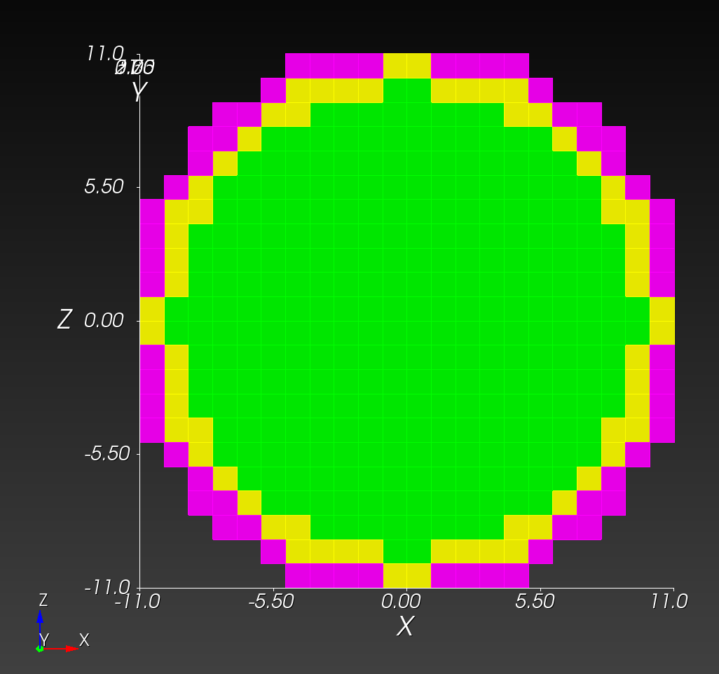 | 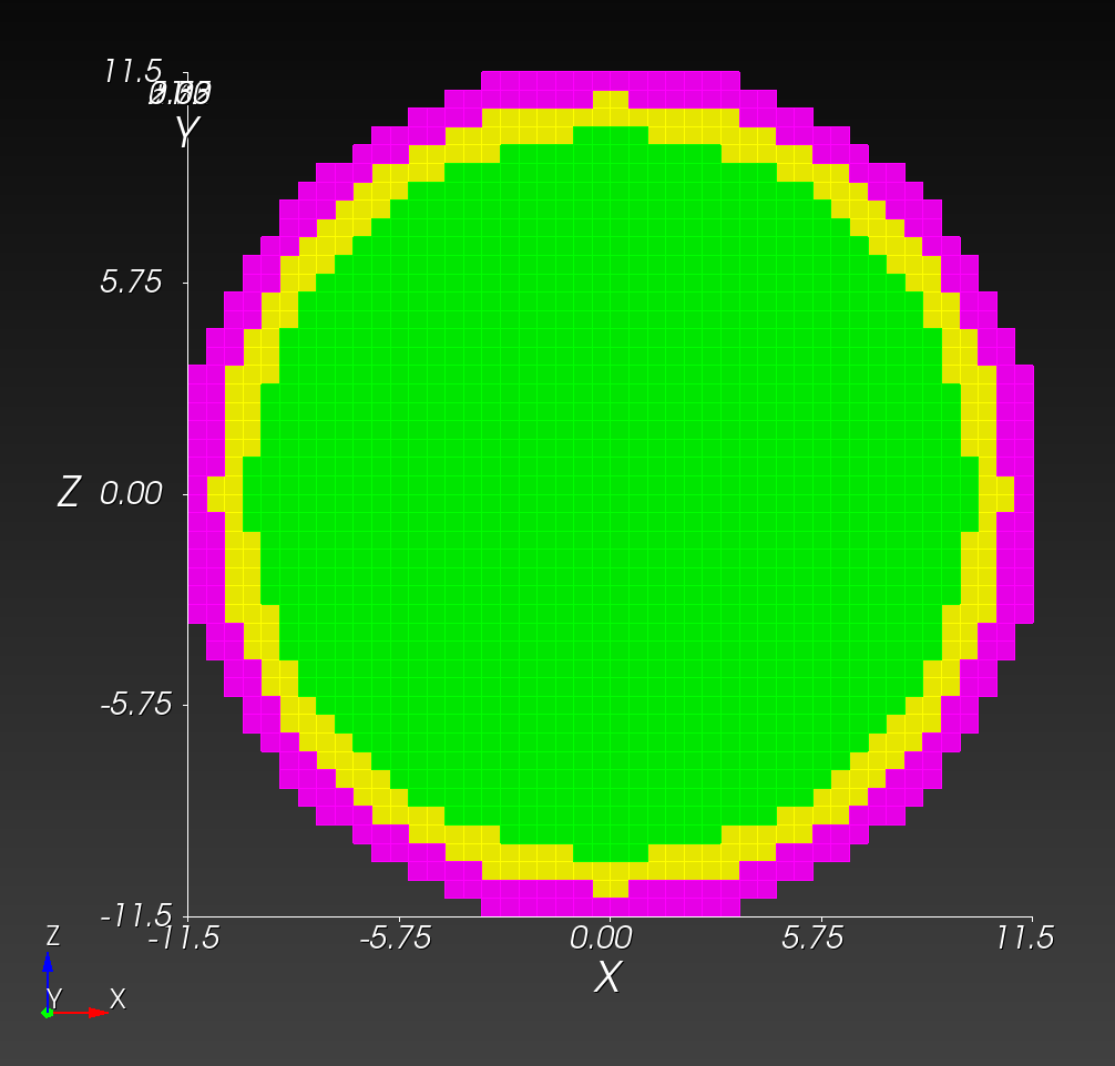 | 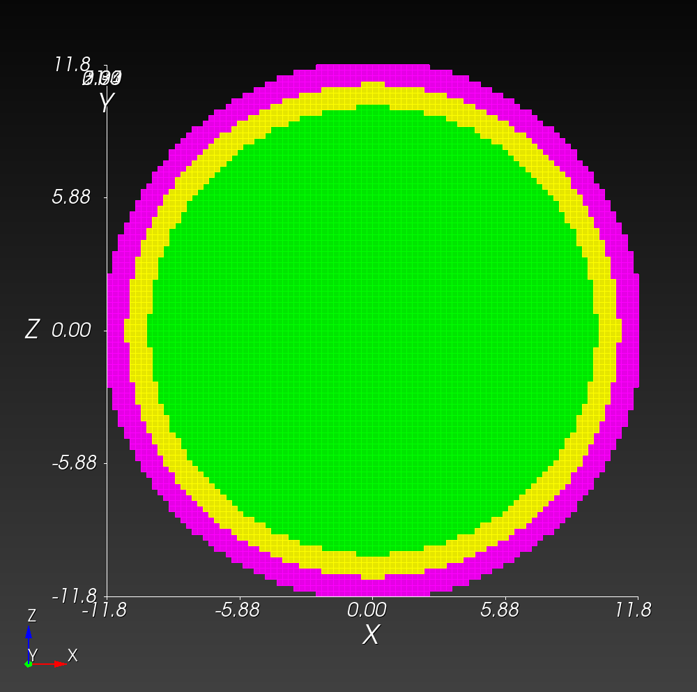 | 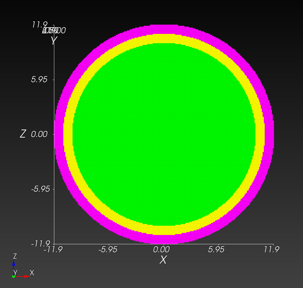 |
| isometric | 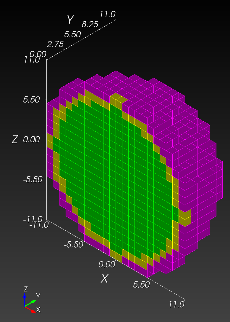 | 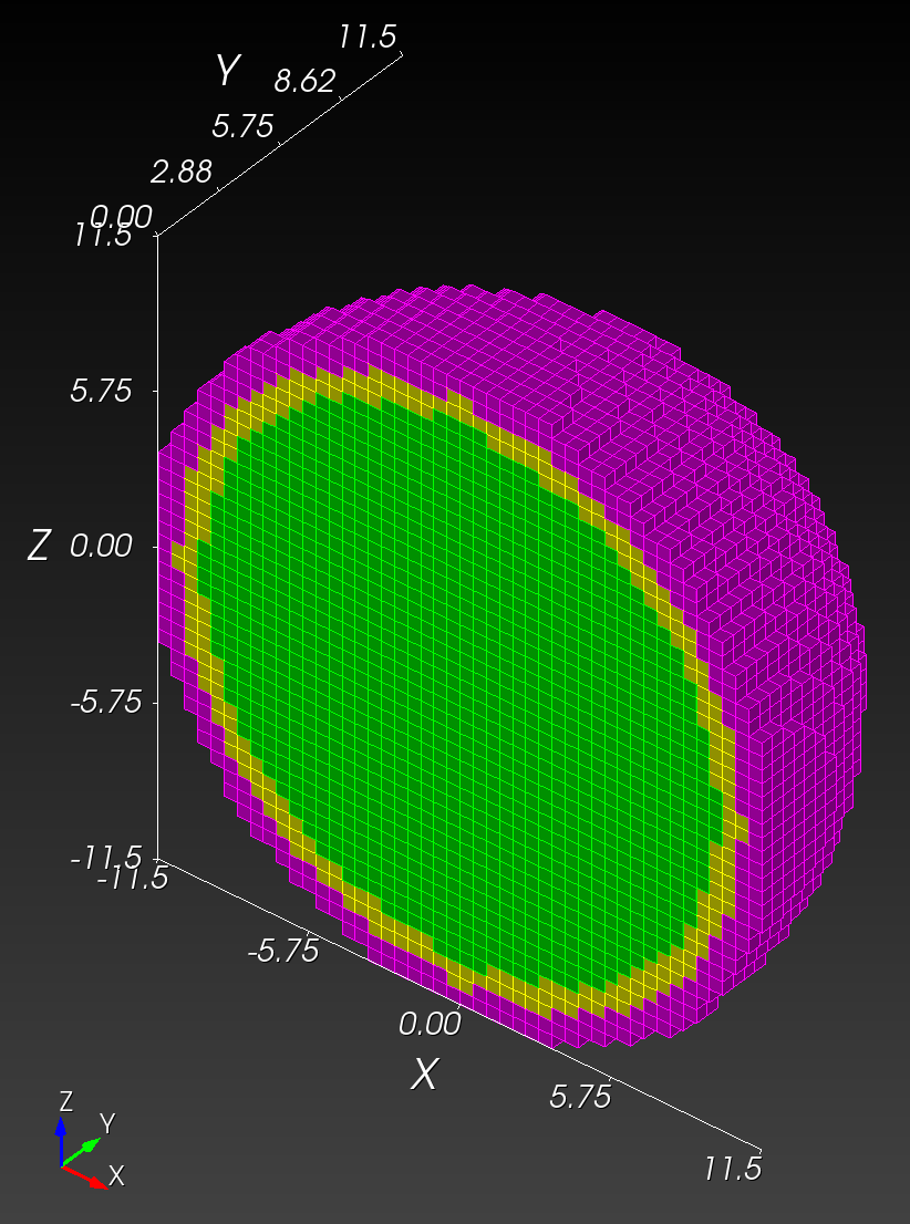 | 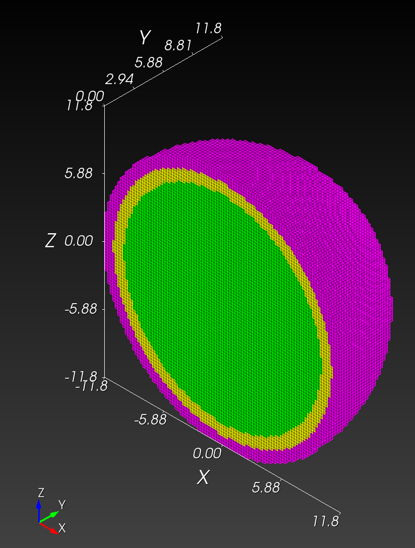 | 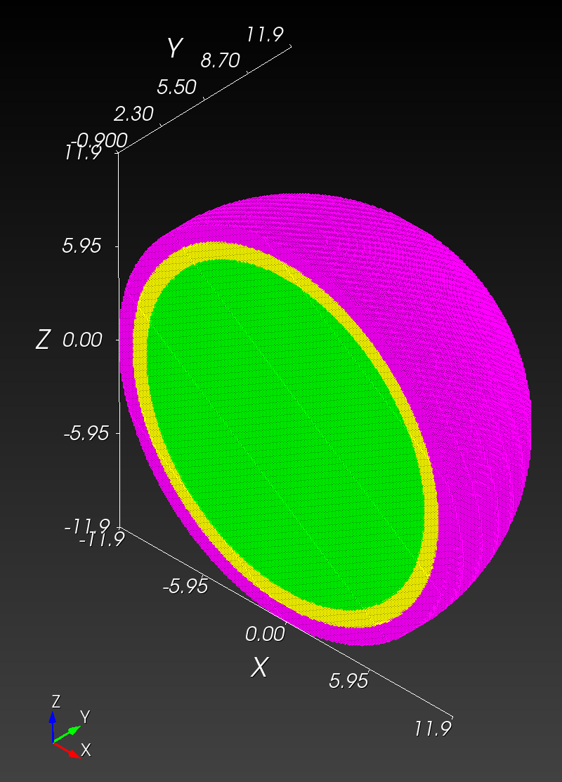 |
| block 1 (green) #elements | 3,648 | 31,408 | 259,408 | 4,136,832 |
| block 2 (yellow) #elements | 1,248 | 10,400 | 86,032 | 1,369,056 |
| block 3 (magenta) #elements | 1,376 | 12,280 | 103,240 | 1,639,992 |
| total #elements | 6,272 | 54,088 | 448,680 | 7,145,880 |
| Exodus file | spheres_resolution_1.exo (401 kB) | spheres_resolution_2.exo (3.2 MB) | spheres_resolution_3.exo (25.7 MB) | spheres_resolution_4.exo (404 MB) |
| Abaqus file | spheres_resolution_1.inp (962 kB) | spheres_resolution_2.inp (8.5 MB) | spheres_resolution_3.inp (73.6 MB) | spheres_resolution_4.inp (1.23 GB) |
Timing - Sculpt
Set up an alias, if needed.
alias sculpt='/Applications/Cubit-16.14/Cubit.app/Contents/MacOS/sculpt'
cd ~/autotwin/automesh/book/analysis/sphere_with_shells/
Use automesh to create .spn files from the .npy files.
automesh convert segmentation -i spheres_resolution_1.npy -o spheres_resolution_1.spn
automesh convert segmentation -i spheres_resolution_2.npy -o spheres_resolution_2.spn
automesh convert segmentation -i spheres_resolution_3.npy -o spheres_resolution_3.spn
automesh convert segmentation -i spheres_resolution_4.npy -o spheres_resolution_4.spn
Run Sculpt.
sculpt --num_procs 1 --input_spn "spheres_resolution_1.spn" \
-x 24 -y 24 -z 24 \
--xtranslate -24 --ytranslate -24 --ztranslate -24 \
--spn_xyz_order 0 \
--exodus_file "spheres_resolution_1" \
--stair 3
Total Time on 1 Procs 0.122201 sec. (0.002037 min.)
sculpt --num_procs 1 --input_spn "spheres_resolution_2.spn" \
-x 48 -y 48 -z 48 \
--xscale 0.5 --yscale 0.5 --zscale 0.5 \
--xtranslate -12 --ytranslate -12 --ztranslate -12 \
--spn_xyz_order 0 \
--exodus_file "spheres_resolution_2" \
--stair 3
Total Time on 1 Procs 0.792997 sec. (0.013217 min.)
sculpt --num_procs 1 --input_spn "spheres_resolution_3.spn" \
-x 96 -y 96 -z 96 \
--xscale 0.25 --yscale 0.25 --zscale 0.25 \
--xtranslate -12 --ytranslate -12 --ztranslate -12 \
--spn_xyz_order 0 \
--exodus_file "spheres_resolution_3" \
--stair 3
Total Time on 1 Procs 7.113380 sec. (0.118556 min.)
sculpt --num_procs 1 --input_spn "spheres_resolution_4.spn" \
-x 240 -y 240 -z 240 \
--xscale 0.1 --yscale 0.1 --zscale 0.1 \
--xtranslate -12 --ytranslate -12 --ztranslate -12 \
--spn_xyz_order 0 \
--exodus_file "spheres_resolution_4" \
--stair 3
Total Time on 1 Procs 135.636523 sec. (2.260609 min.)
The table below summarizes the relative processing times, Sculpt versus automesh (completed with automesh version 0.2.9)
| resolution | 1 vox/cm | 2 vox/cm | 4 vox/cm | 10 vox/cm |
|---|---|---|---|---|
automesh | 1 | 1 | 1 | 1 |
| Sculpt | 6.73 | 31.6 | 97.8 | 141 |
Simulation
Work in progress.
Meshes
Copy from local to HPC:
# for example, manual copy from local to HPC
# macOS local finder, command+K to launch "Connect to Server"
# smb://cee/chovey
# copy [local]~/autotwin/automesh/book/analysis/sphere_with_shells/spheres_resolution_2.exo
# to
# [HPC]~/autotwin/ssm/geometry/sr2/
We consider three simulations using the following three meshes (in the HPC ~/autotwin/ssm/geometry folder):
| folder | file | md5 checksum |
|---|---|---|
sr2 | spheres_resolution_2.exo | 9f40c8bd91874f87e22a456c76b4448c |
sr3 | spheres_resolution_3.exo | 6ae69132897577e526860515e53c9018 |
sr4 | spheres_resolution_4.exo | b939bc65ce07d3ac6a573a4f1178cfd0 |
We do not use the spheres_resolution_1.exo because the outer shell layer is not closed.
Boundary Conditions
Consider an angular acceleration pulse of the form:
and is zero otherwise. This pulse, referred to as the bump function, is continuously differentiable, with peak angular acceleration at .
With krad/s^2, and ms, we can create the angular acceleration boundary condition (with corresponding angular velocity) 1 plots:
| Angular Acceleration | Angular Velocity |
|---|---|
 |  |
Figure 6.1.3-1: Angular acceleration and corresponding angular velocity time history.
- Angular acceleration tabulated data: The standardized angular acceleration load curve has column data as (time, magnitude) in (sec, krad/s^2). The function used to generated the curve, from Equation (1) of 1, is
- Angular velocity tabulated data: The angular velocity curve has column data as (time, magnitude) in (sec, rad/s).
The peak angular acceleration occurs at (which occurs in the tabular data at data point 4144, values (0.00414310, 7.99999997)).
On the outer shell (block 3) of the model, we prescribe the angular velocity boundary condition.
Tracers
View the tracer locations in Cubit:
graphics clip on plane location 0 0 1 direction 0 0 -1
view up 0 1 0
view from 0 0 100
graphics clip manipulation off
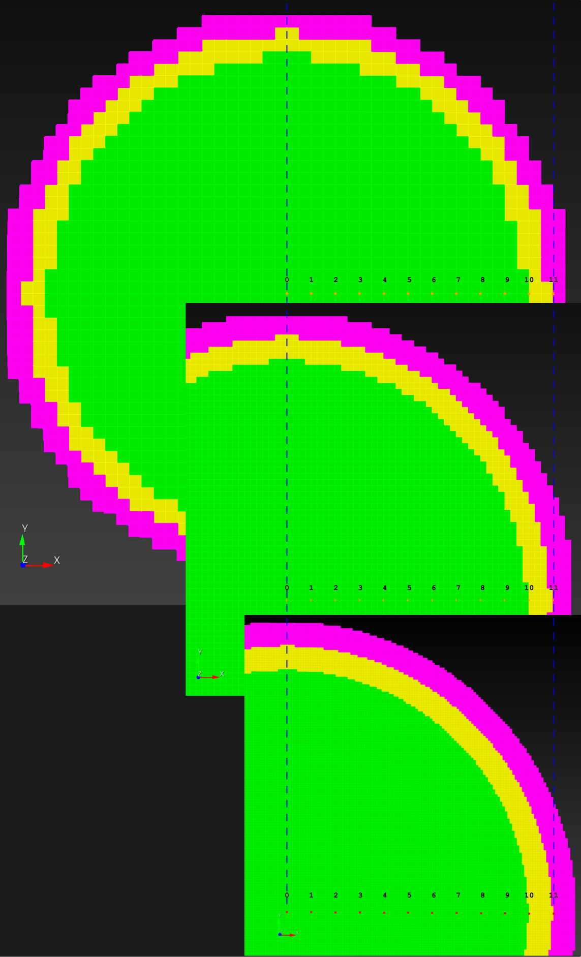
Figure 6.1.3-2: Tracer numbers [0, 1, 2, ... 11] at distance [0, 1, 2, ... 11] centimeters from point (0, 0, 0) along the x-axis at resolutions sr2, sr3, and sr4 (top to bottom, respectively).
Materials
We model the outer shell (block 3) as a rigid body. The inner sphere (block 1) is modeled as Swanson viscoelastic white matter. The intermediate material (block 2) is modeled as elastic cerebral spinal fluid.
Input deck
We created three input decks:
sr2.i(for meshspheres_reolution_2.exo)sr3.i(for meshspheres_reolution_3.exo)sr4.i(for meshspheres_reolution_4.exo)
Remark: Originally, we used APREPRO, part of SEACAS, to define tracer points along the line at 1-cm (radial) intervals. We then updated the locations of these tracer points to be along the x-axis, which allowed for nodally exact locations to be established across all models, voxelized and conforming.
Displacement, maximum principal log strain, and maximum principal rate of deformation were logged at tracer points over the simulation duration. The Sierra/Solid Mechanics documentation 2 3 was also useful for creating the input decks.
Solver
Request resources:
mywcid # see what wcid resources are available, gives an FYxxxxxx number
#request 1 interactive node for four hours with wcid account FY180100
salloc -N1 --time=4:00:00 --account=FY180100
See idle nodes:
sinfo
Decompose the geometry, e.g., ~/autotwin/ssm/geometry/sr2/submit_script:
#!/bin/bash

module purge
module load sierra
module load seacas

# previously ran with 16 processors
# PROCS=16
# 10 nodes = 160 processors
PROCS=160
# PROCS=320
# PROCS=336

# geometry and mesh file
GFILE="spheres_resolution_2.exo"

decomp --processors $PROCS $GFILE
Check the input deck ~/autotwin/ssm/input/sr2/sr2.i with submit_check:
#!/bin/bash

echo "This is submit_check"
echo "module purge"
module purge

echo "module load sierra"
module load sierra

# new, run this first
export PSM2_DEVICES='shm,self'

IFILE="sr2.i"

echo "Check syntax of input deck: $IFILE"
adagio --check-syntax -i $IFILE  # to check syntax of input deck

# echo "Check syntax of input deck ($IFILE) and mesh loading"
adagio --check-input  -i $IFILE  # to check syntax of input deck and mesh load
Clean any preexisting result files with submit_clean:
#!/bin/bash

echo "This is submit_clean"
rm batch_*
rm sierra_batch_*
rm *.e.*
rm epu.log
rm *.g.*
rm *.err
rm g.rsout.*
Submit the job with submit_script:
#!/bin/bash

echo "This is submit_script"
module purge
module load sierra
module load seacas

# PROCS=16
PROCS=160
# PROCS=320
# PROCS=336

# geometry and mesh file
# GFILE="../../geometry/sphere/spheres_resolution_4.exo"
# decomp --processors $PROCS $GFILE

IFILE="sr2.i"

# queues
# https://wiki.sandia.gov/pages/viewpage.action?pageId=1359570410#SlurmDocumentation-Queues
# short can be used for nodes <= 40 and wall time <= 4:00:00 (4 hours)
# batch, the default queue, wall time <= 48 h
# long, wall time <= 96 h, eclipse 256 nodes

# https://wiki.sandia.gov/display/OK/Slurm+Documentation
# over 4 hours, then need to remove 'short' from the --queue-name
#
# sierra -T 00:20:00 --queue-name batch,short --account FY180042 -j $PROCS --job-name $IFILE --run adagio -i $IFILE
sierra -T 04:00:00 --queue-name batch,short --account FY180042 -j $PROCS --job-name $IFILE --run adagio -i $IFILE
# sierra -T 06:00:00 --queue-name batch --account FY180042 -j $PROCS --job-name $IFILE --run adagio -i $IFILE
# sierra -T 24:00:00 --queue-name batch --account FY180042 -j $PROCS --job-name $IFILE --run adagio -i $IFILE
Monitor the job:
# monitoring
squeue -u chovey
tail foo.log
tail -f foo.log # interactive monitor
Add shortcuts, if desired, to the ~/.bash_profile:
alias sq="squeue -u chovey"
alias ss="squeue -u chovey --start"
Cancel the job:
scancel JOB_ID
scancel -u chovey # cancel all jobs
Compute time:
| item | sim | T_sim (ms) | HPC | #proc | cpu time (hh:mm) |
|---|---|---|---|---|---|
| 0 | sr2.i | 20 | att | 160 | less than 1 min |
| 1 | sr3.i | 20 | att | 160 | 00:04 |
| 2 | sr4.i | 20 | ecl | 160 | 03:58 |
Results
Copy the files, history_rigid.csv and history.csv, which contain tracer rigid and deformable body time histories, from the HPC to the local.
Rigid Body
With figio and the rigid_body_ang_kinematics.yml recipe,
cd ~/autotwin/automesh/book/analysis/sphere_with_shells/recipes
figio rigid_body_ang_kinematics.yml
verify that the rigid body input values were successfully reflected in the output:
| angular acceleration | angular velocity | angular position |
|---|---|---|
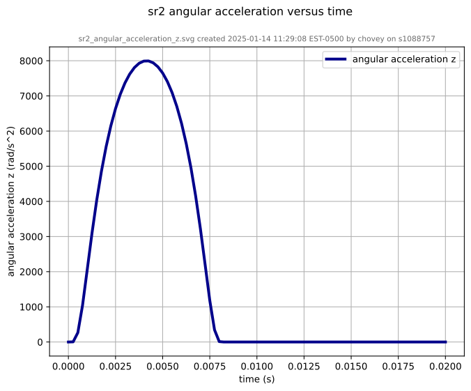 | 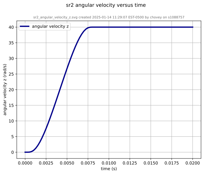 | 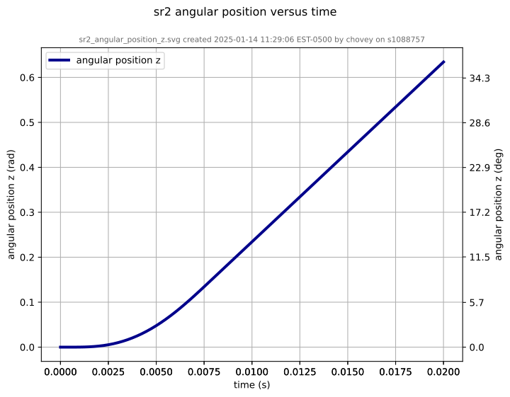 |
Figure 6.1.3-3: Rigid body (block 3) kinematics for sr2, the sphere_resolution_2.exo model. The time history traces appear the same for the sr3 and sr4 models.
Deformable Body
The following figure shows the maximum principal log strain for various resolutions and selected times.
| resolution | 2 vox/cm | 4 vox/cm | 10 vox/cm |
|---|---|---|---|
| midline | | | |
| t=0.000 s |  | |  |
| t=0.002 s | 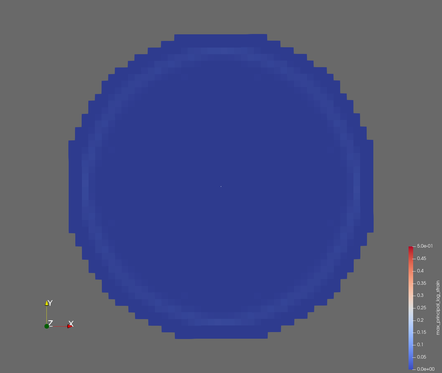 | 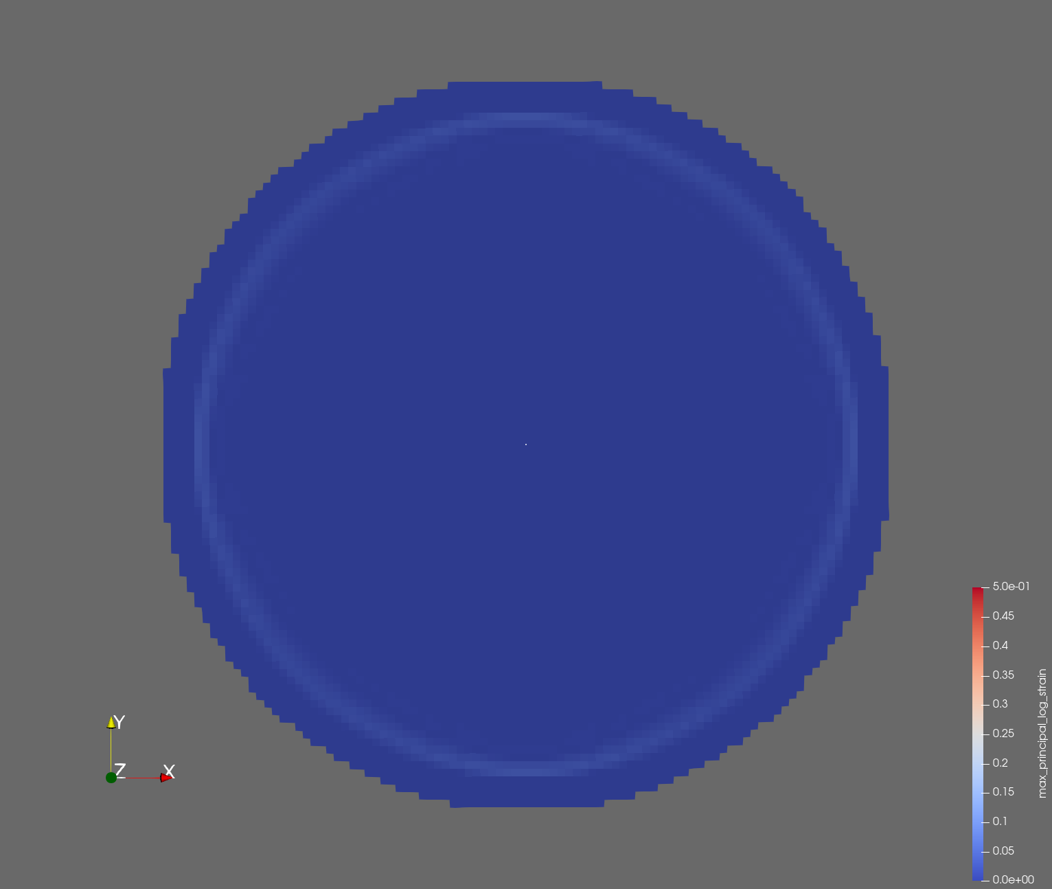 |  |
| t=0.004 s | 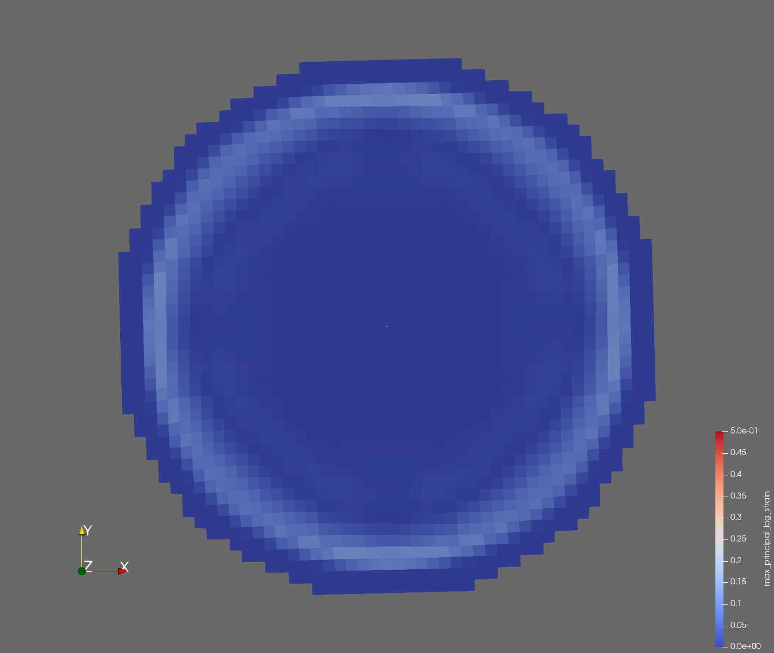 | 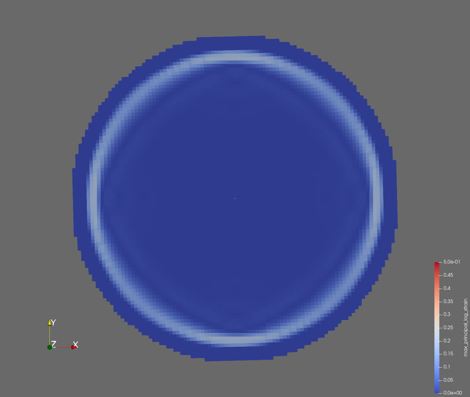 |  |
| t=0.006 s | 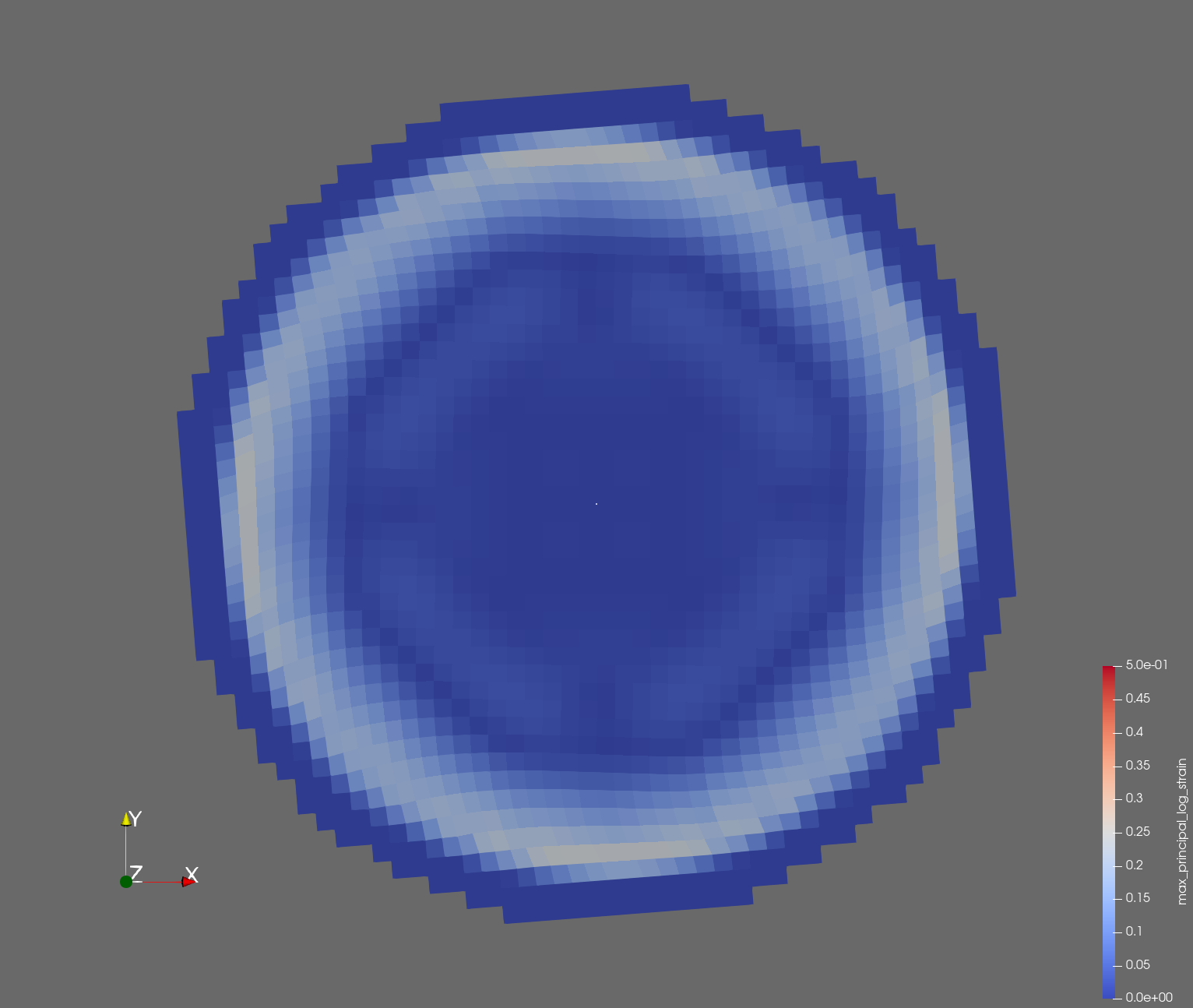 | 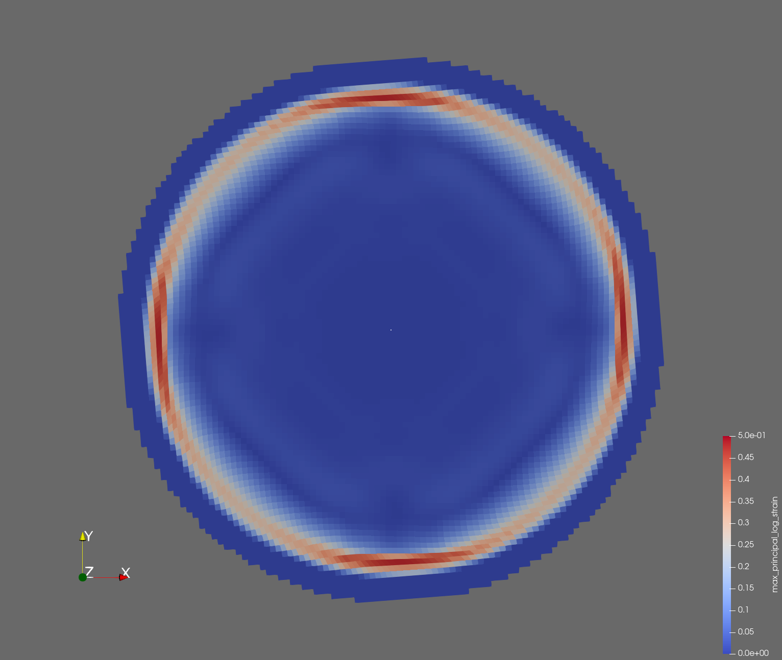 |  |
| t=0.008 s | 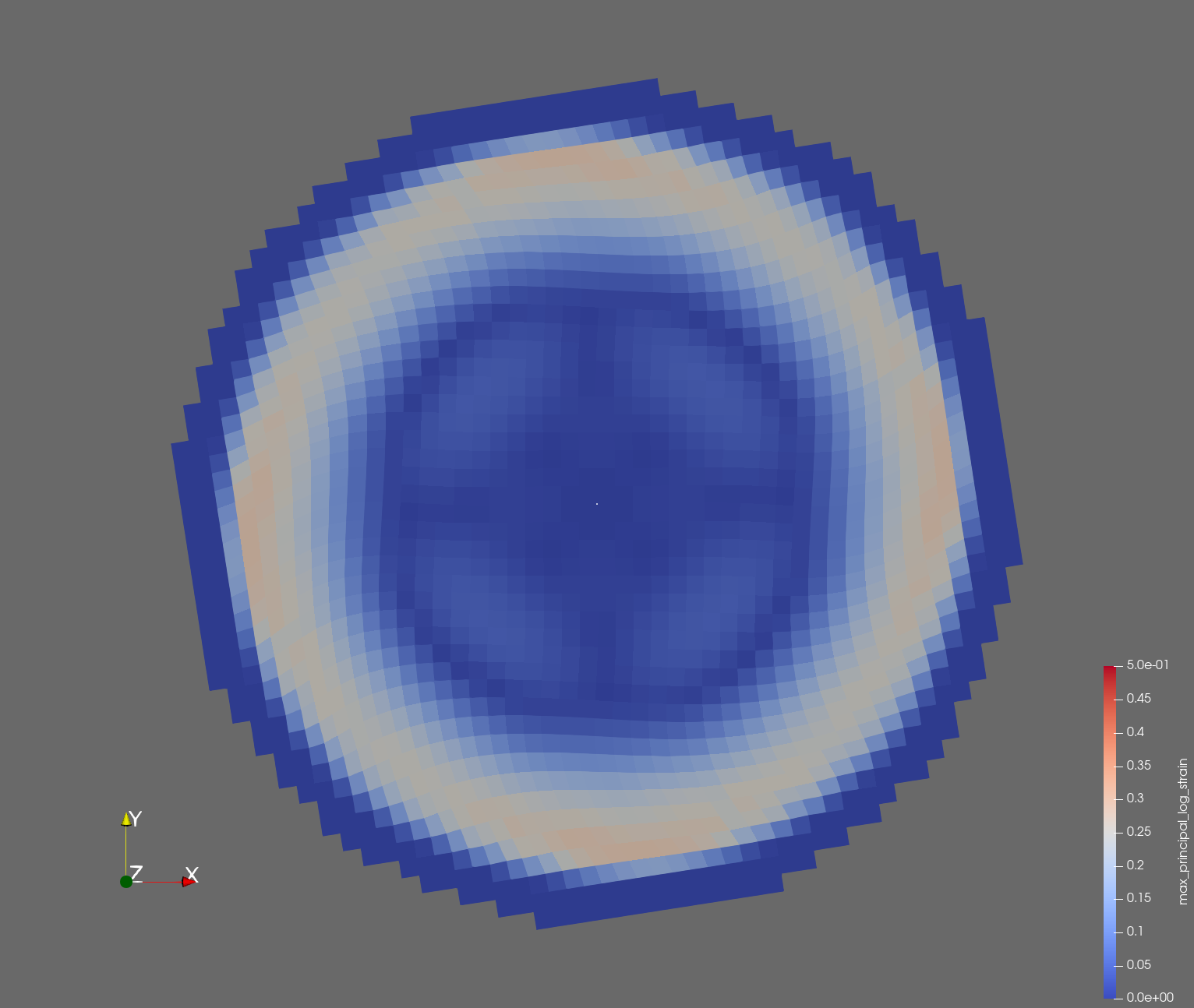 | 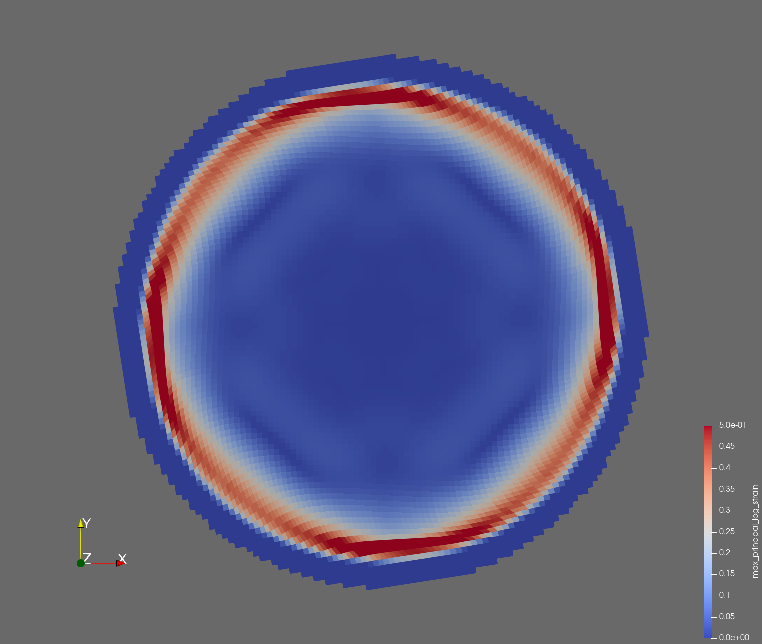 |  |
| t=0.010 s | 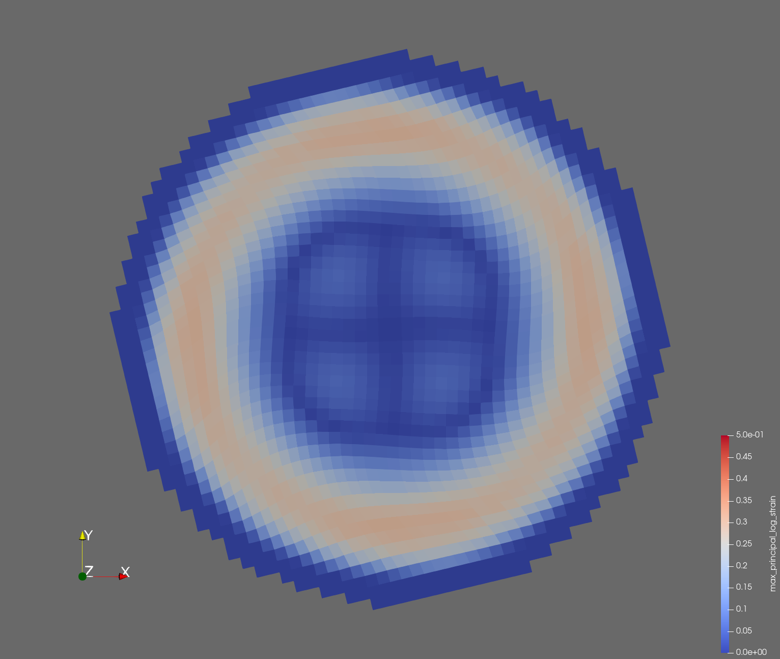 | 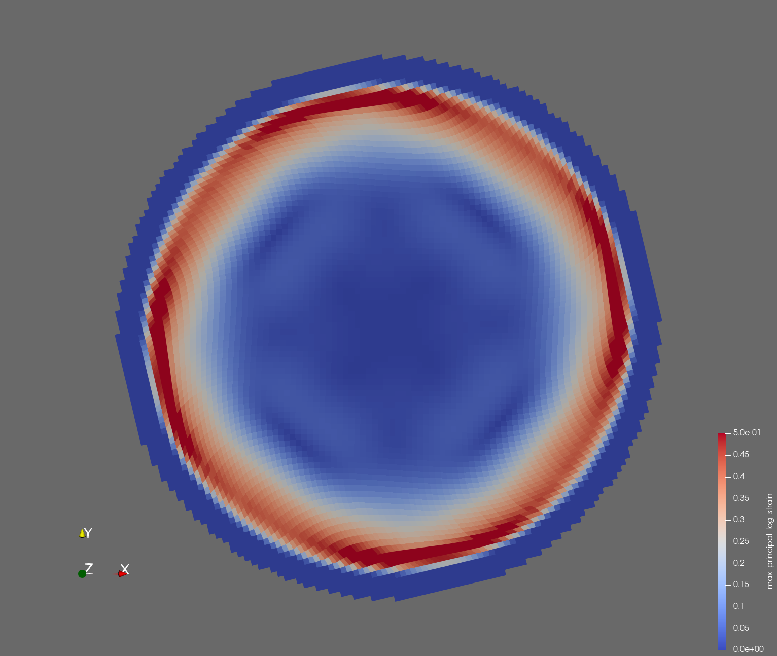 |  |
| t=0.012 s | 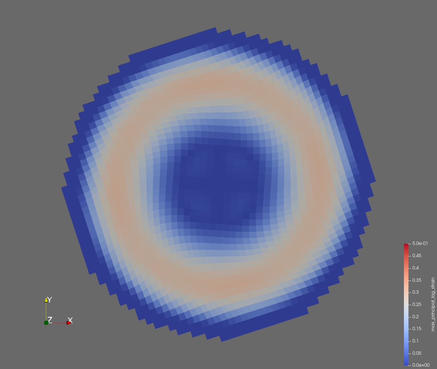 | 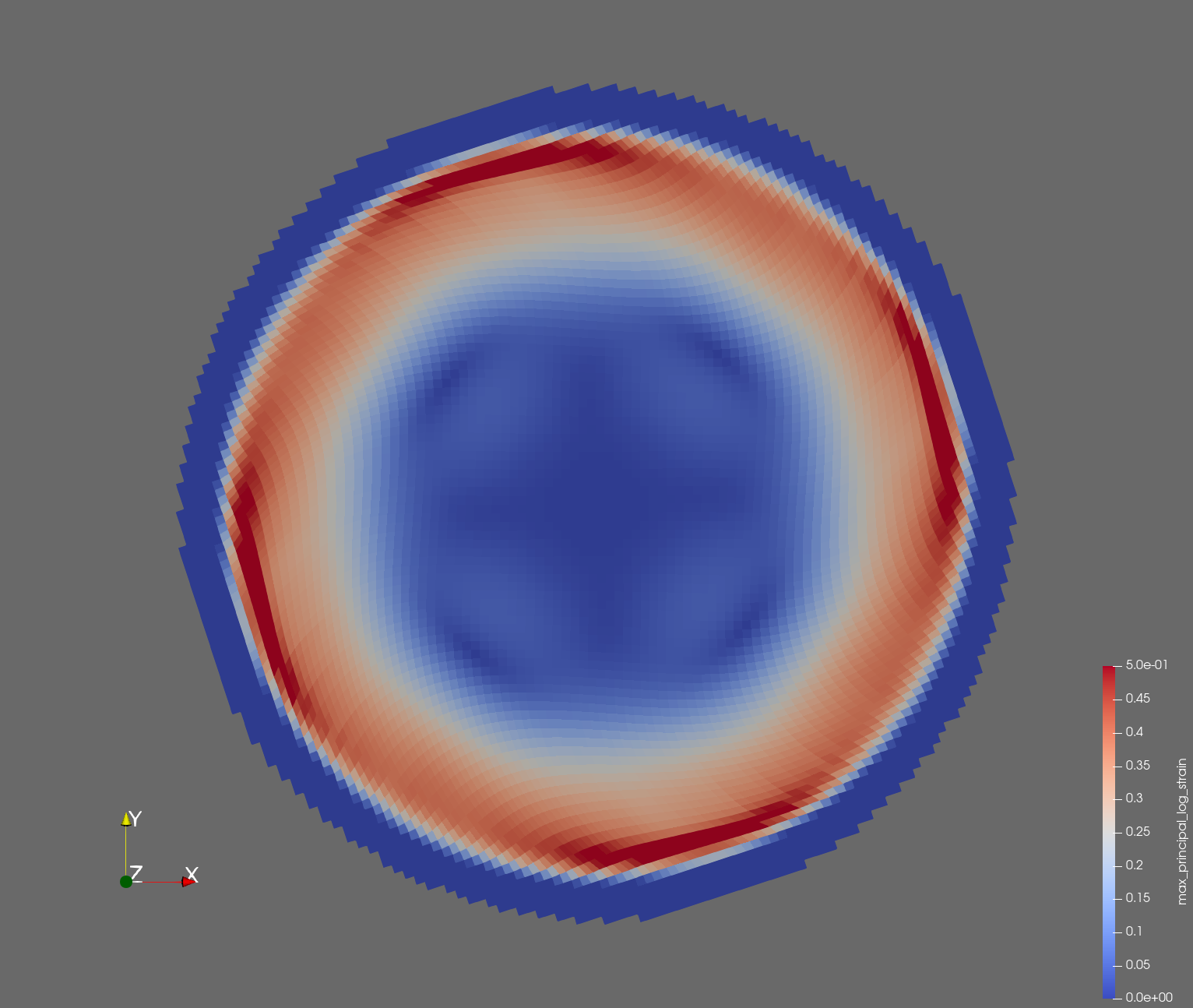 |  |
| t=0.014 s |  |  |  |
| t=0.016 s |  |  |  |
| t=0.018 s | 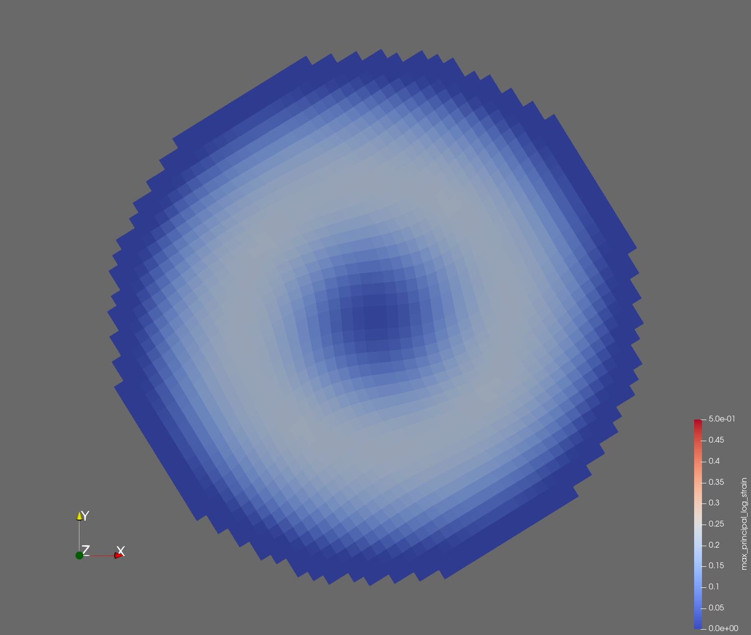 | 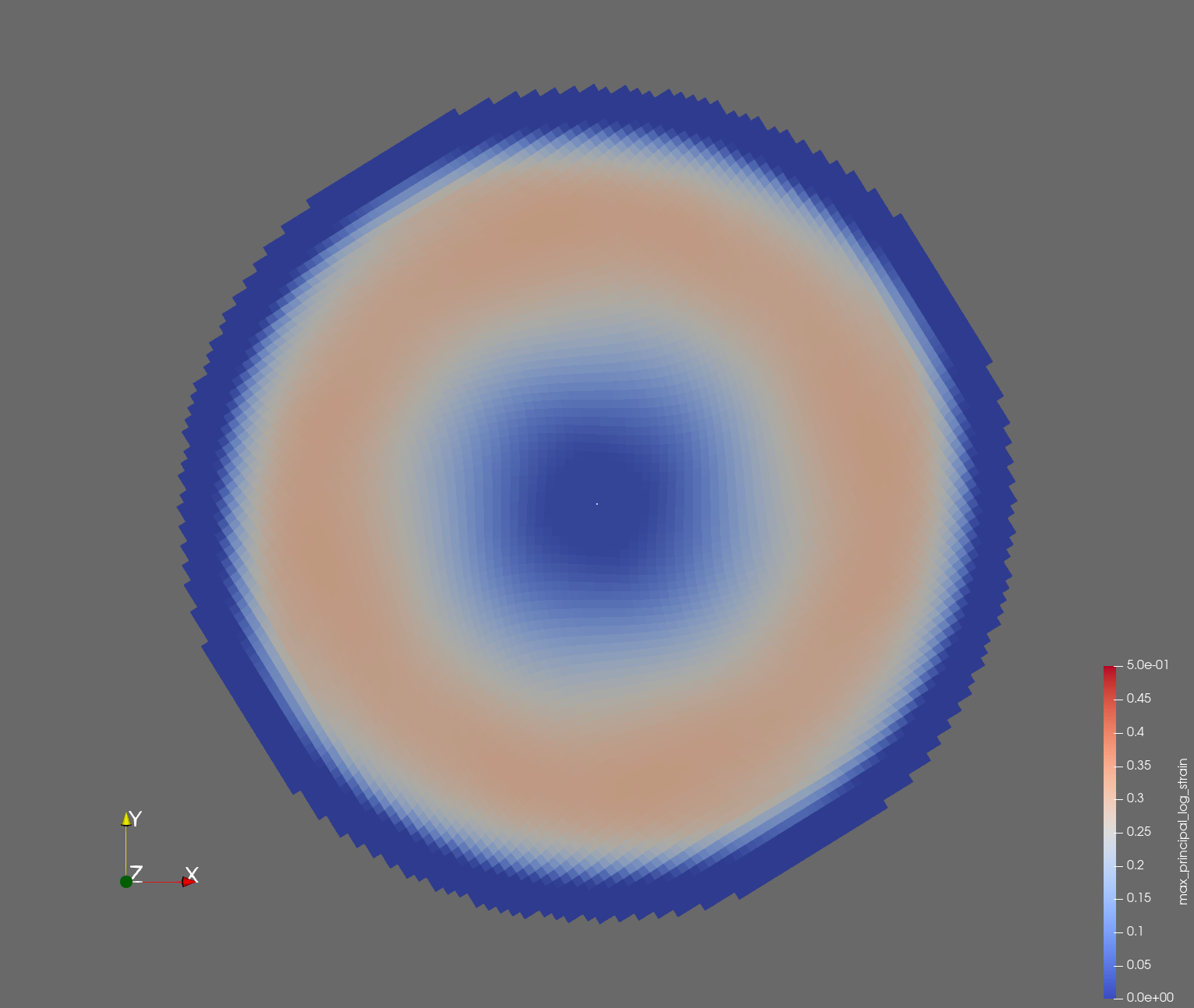 |  |
| t=0.020 s | 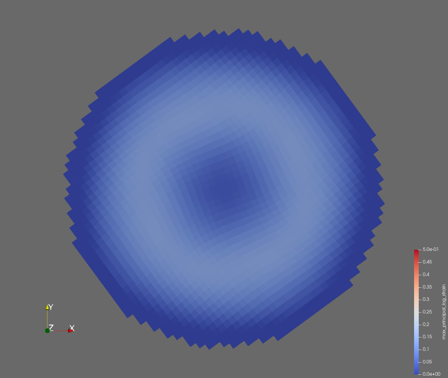 | 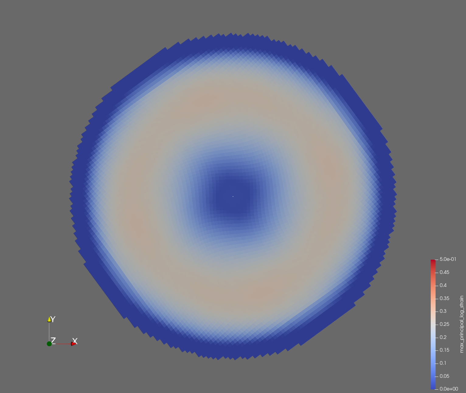 |  |
| displacement | 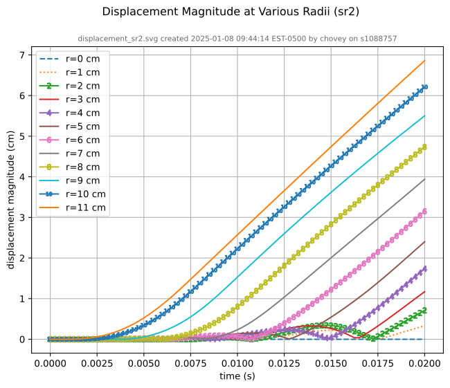 | 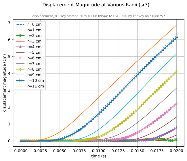 | 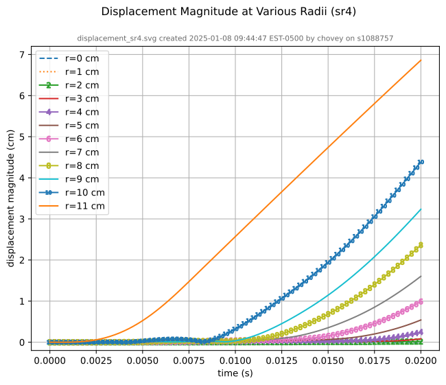 |
| recipe | displacement_sr2.yml | displacement_sr3.yml | displacement_sr4.yml |
| log strain | 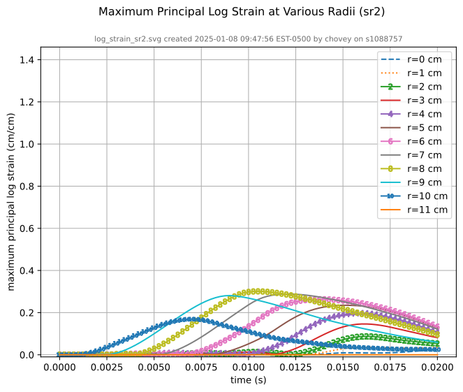 |  |  |
| recipe | log_strain_sr2.yml | log_strain_sr3.yml | log_strain_sr4.yml |
| rate of deformation |  |  | 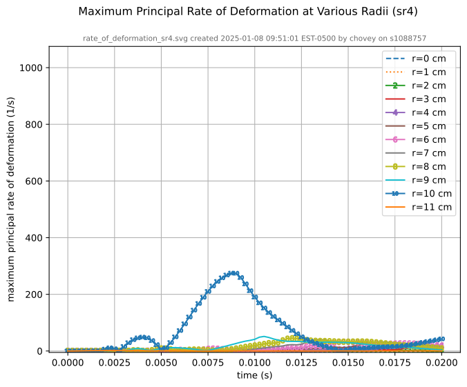 |
| recipe | rate_of_deformation_sr2.yml | rate_of_deformation_sr3.yml | rate_of_deformation_sr4.yml |
Figure 6.1.3-4: Voxel mesh midline section, with contour plot of maximum principal log strain at selected times from 0.000 s to 0.020 s (1,000 Hz sample rate, = 0.001 s), and tracer plots at 1 cm interval along the -axis for displacement magnitude, log strain, and rate of deformation (4,000 Hz acquisition rate, = 0.00025 s).
References
-
Carlsen RW, Fawzi AL, Wan Y, Kesari H, Franck C. A quantitative relationship between rotational head kinematics and brain tissue strain from a 2-D parametric finite element analysis. Brain Multiphysics. 2021 Jan 1;2:100024. paper ↩ ↩2
-
Beckwith FN, Bergel GL, de Frias GJ, Manktelow KL, Merewether MT, Miller ST, Parmar KJ, Shelton TR, Thomas JD, Trageser J, Treweek BC. Sierra/SolidMechanics 5.10 Theory Manual. Sandia National Lab. (SNL-NM), Albuquerque, NM (United States); Sandia National Lab. (SNL-CA), Livermore, CA (United States); 2022 Sep 1. link ↩
-
Thomas JD, Beckwith F, Buche MR, de Frias GJ, Gampert SO, Manktelow K, Merewether MT, Miller ST, Mosby MD, Parmar KJ, Rand MG, Schlinkman RT, Shelton TR, Trageser J, Treweek B, Veilleux MG, Wagman EB. Sierra/SolidMechanics 5.22 Example Problems Manual. Sandia National Lab. (SNL-NM), Albuquerque, NM (United States); Sandia National Lab. (SNL-CA), Livermore, CA (United States); 2024 Oct 1. link ↩
Conforming Mesh
In this section, we develop a traditional conforming mesh, manually constructed with Cubit. We compare the results from the conforming resolutions to the results obtained from the voxel mesh resolutions.
Mesh Creation and Visualization
With conforming_spheres.jou in Cubit, we create three conforming meshes to match the three voxel meshes of resolution 0.5, 0.25, and 0.1 cm (2 vox/cm, 4 vox/cm, and 10 vox/cm, respectively).
| resolution | 2 vox/cm | 4 vox/cm | 10 vox/cm |
|---|---|---|---|
| midline | 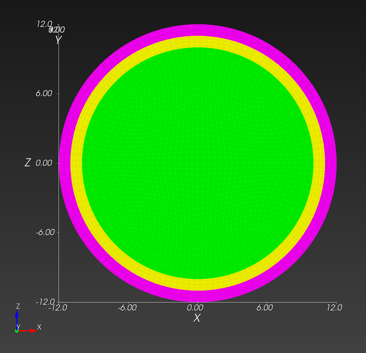 | 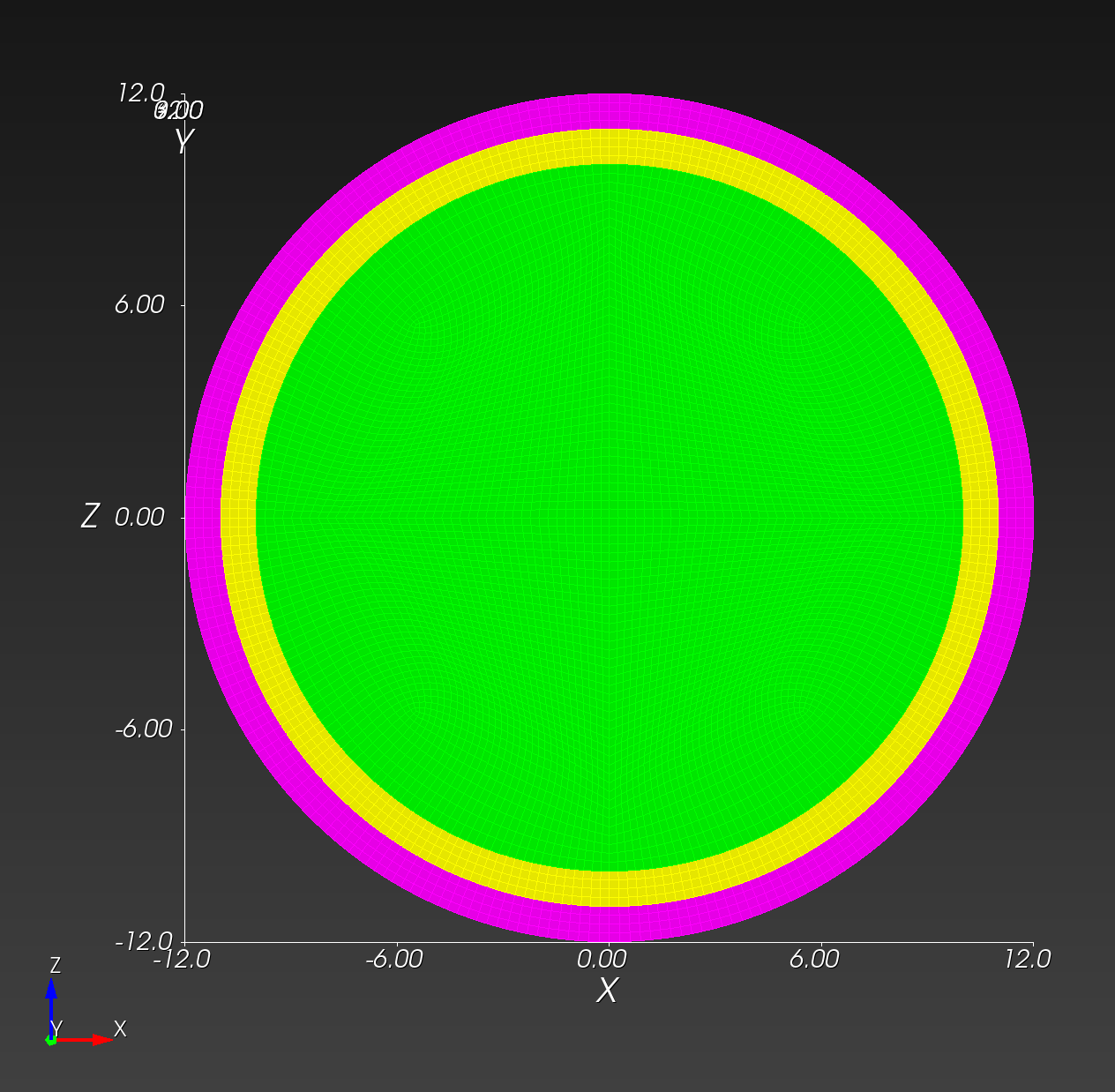 | 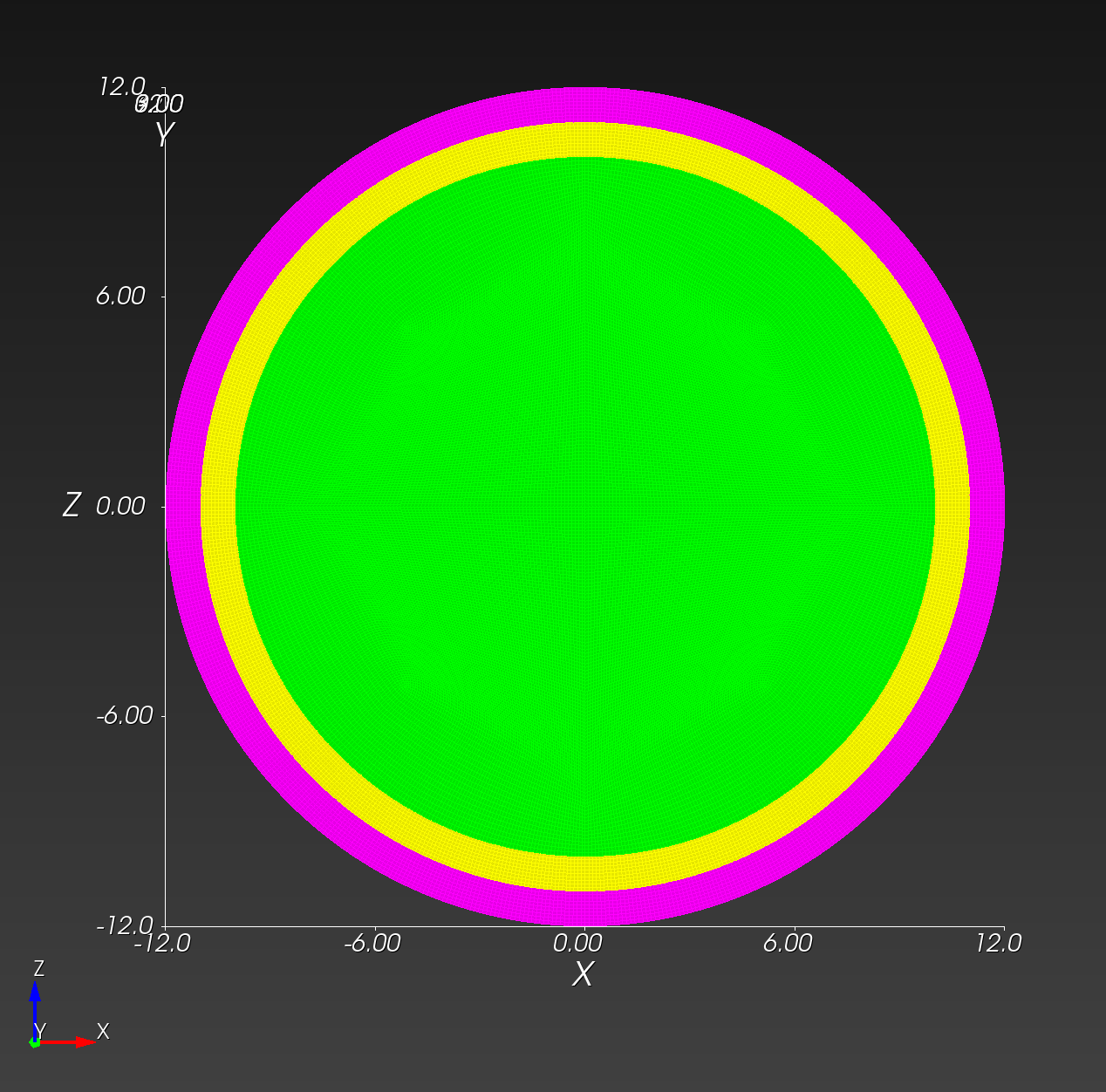 |
| isometric | 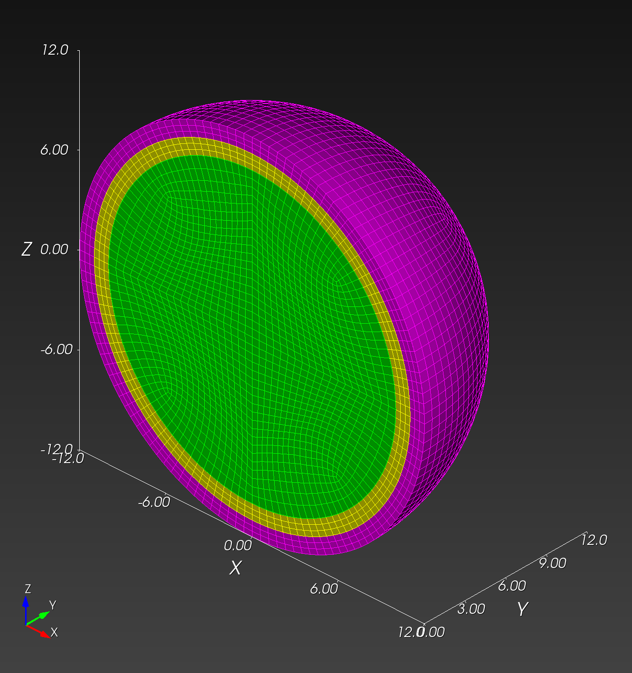 | 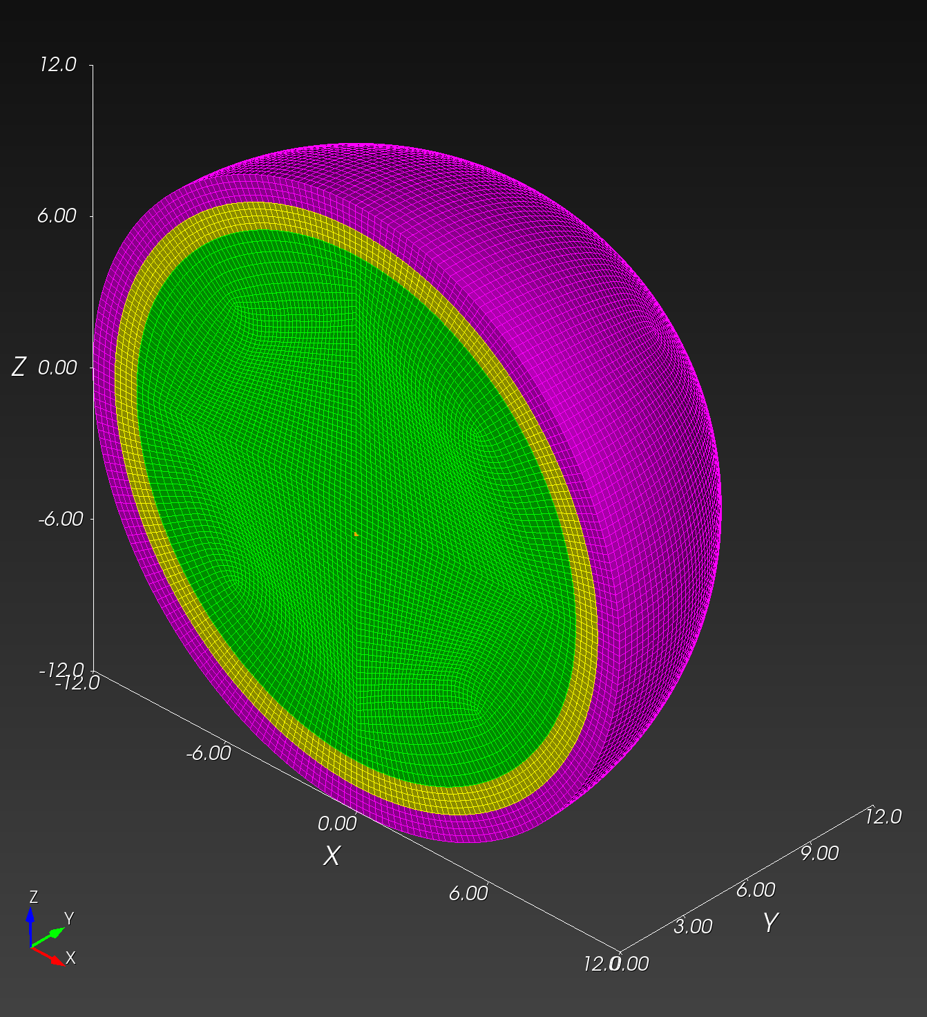 | 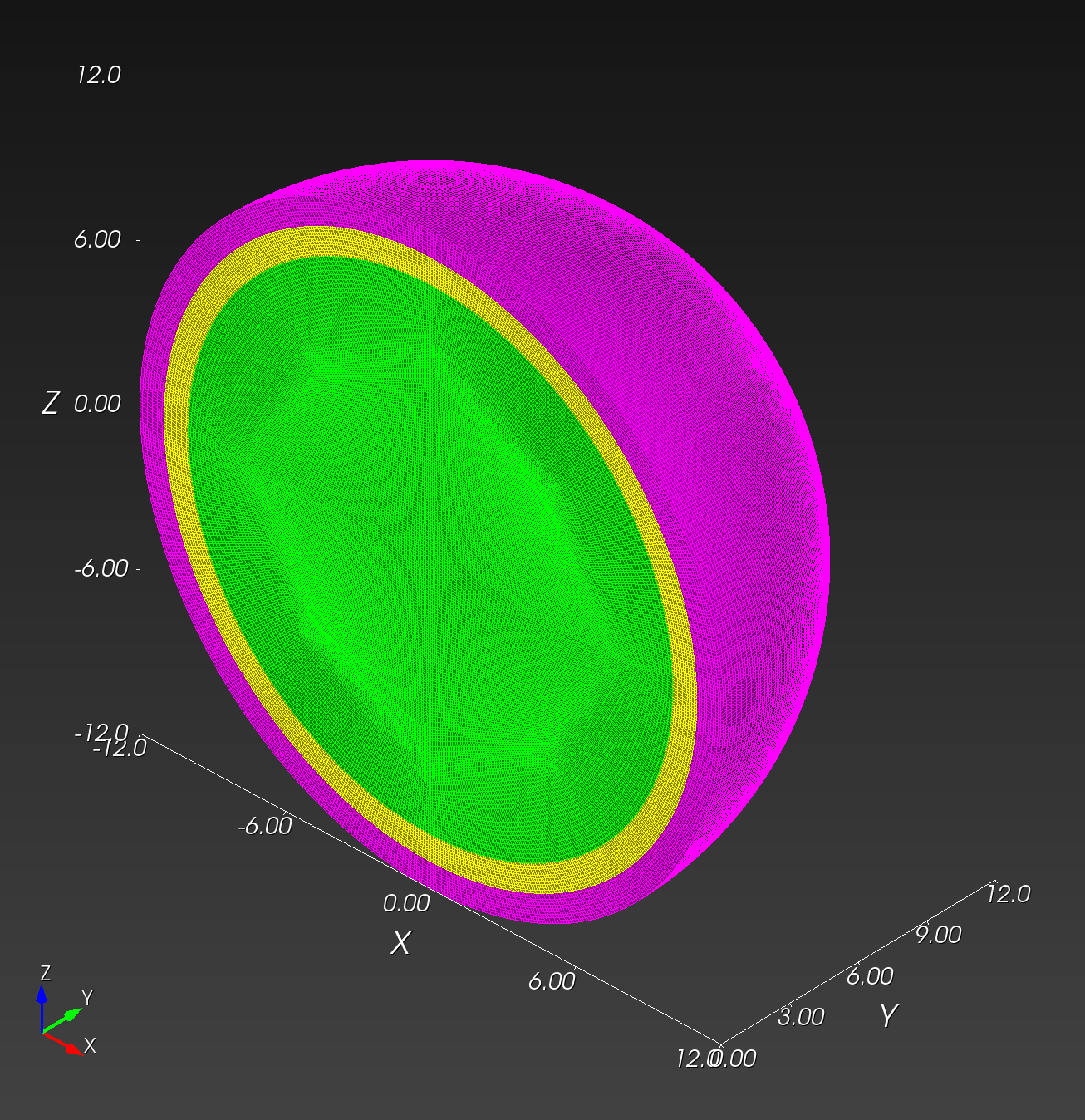 |
| block 1 (green) #elements | 57,344 | 458,752 | 7,089,776 |
| block 2 (yellow) #elements | 18,432 | 98,304 | 1,497,840 |
| block 3 (magenta) #elements | 18,432 | 98,304 | 1,497,840 |
| total #elements | 94,208 | 655,360 | 10,085,456 |
Copy from local to HPC:
# for example, manual copy from local to HPC
# macOS local finder, command+K to launch "Connect to Server"
# smb://cee/chovey
# copy [local]~/autotwin/automesh/book/analysis/sphere_with_shells/conf_0.5cm.g
# to
# [HPC]~/autotwin/ssm/geometry/sr2c/
We consider three simulations using the following three meshes (in the HPC ~/autotwin/ssm/geometry folder or downloadable from the links in the file column below):
| folder | file | md5 checksum | size |
|---|---|---|---|
sr2c | conf_0.5cm.g | 3731460f73da70ae79dd8155e2a8e0c6 | 7 MB |
sr3c | conf_0.25cm.g | bf65e329f43867c8fabc64b1b5273b8c | 47 MB |
sr4c | conf_0.1cm.g | ae0b13dec173c8fb030feab306a09db6 | 700 MB |
Tracers
View the tracer locations in Cubit:
graphics clip on plane location 0 0 1 direction 0 0 -1
view up 0 1 0
view from 0 0 100
graphics clip manipulation off
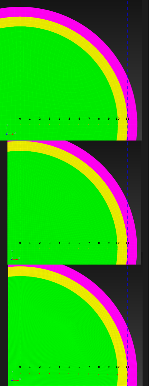
Figure 6.1.4-1: Tracer numbers [0, 1, 2, ... 11] at distance [0, 1, 2, ... 11] centimeters from point (0, 0, 0) along the x-axis at resolutions sr2c, sr3c, and sr4c (top to bottom, respectively).
Simulation
We created three input decks:
Results
Compute time:
| item | sim | T_sim (ms) | HPC | #proc | cpu time (hh:mm) |
|---|---|---|---|---|---|
| 0 | sr2c.i | 20 | gho | 160 | 00:02 |
| 1 | sr3c.i | 20 | gho | 160 | 00:21 |
| 2 | sr4.i | 20 | att | 160 | 14:00 (est) |
Rigid Body
We verified the rigid body kinematics match those from the voxel mesh, but we don't repeat those time history plots here.
Deformable Body
| resolution | 2 vox/cm | 4 vox/cm | 10 vox/cm |
|---|---|---|---|
| midline | | | |
| displacement | 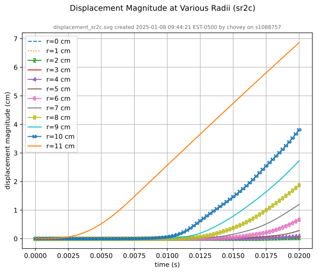 | 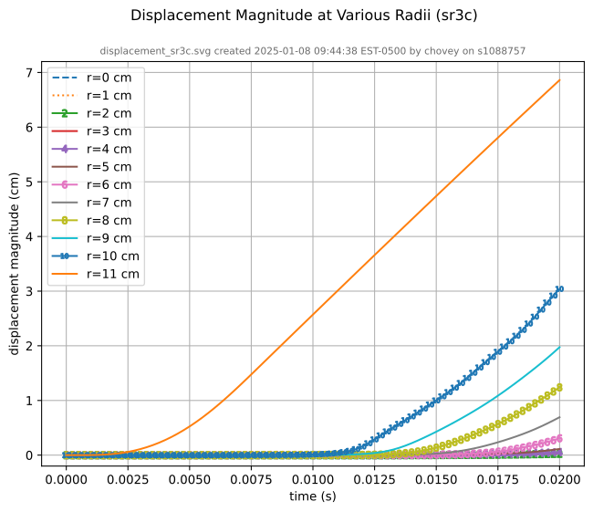 |  |
| recipe | displacement_sr2c.yml | displacement_sr3c.yml | displacement_sr4c.yml |
| log strain | 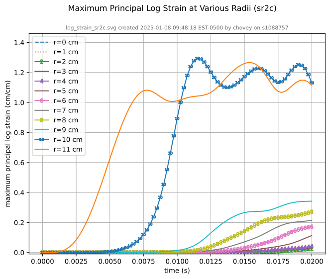 | 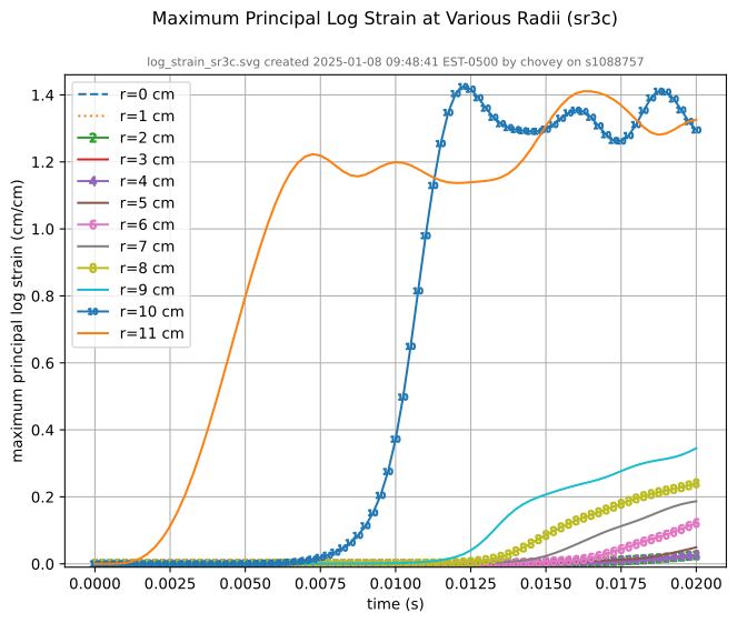 |  |
| recipe | log_strain_sr2c.yml | log_strain_sr3c.yml | log_strain_sr4c.yml |
| rate of deformation | 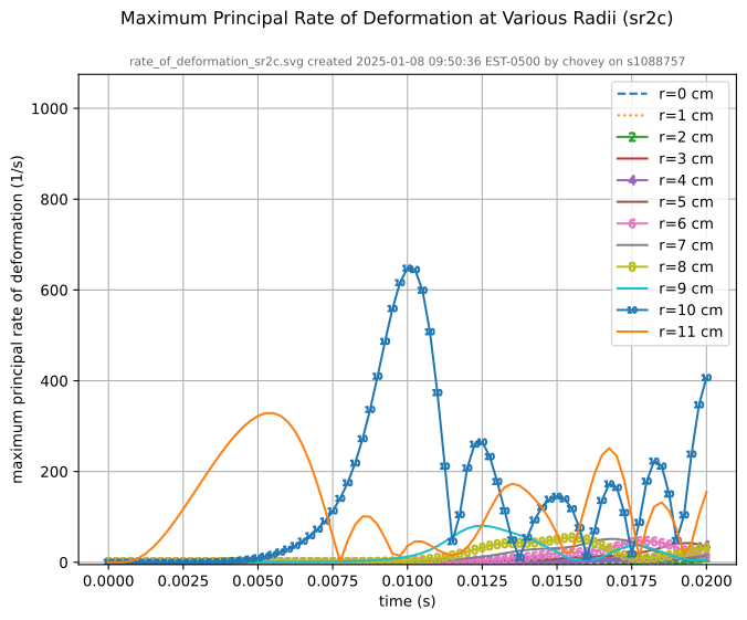 | 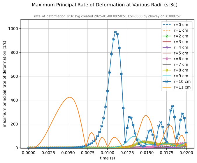 |  |
| recipe | rate_of_deformation_sr2c.yml | rate_of_deformation_sr3c.yml | rate_of_deformation_sr4c.yml |
Figure 6.1.4-2: Conforming mesh midline section and tracer plots at 1 cm interval along the -axis for displacement magnitude, log strain, and rate of deformation (10,000 Hz acquisition rate, = 0.0001 s).
Smoothed Mesh
alias automesh='~/autotwin/automesh/target/release/automesh'
cd ~/autotwin/automesh/book/analysis/sphere_with_shells
Taubin Smoothing
sr2s10 | sr2s50 |
|---|---|
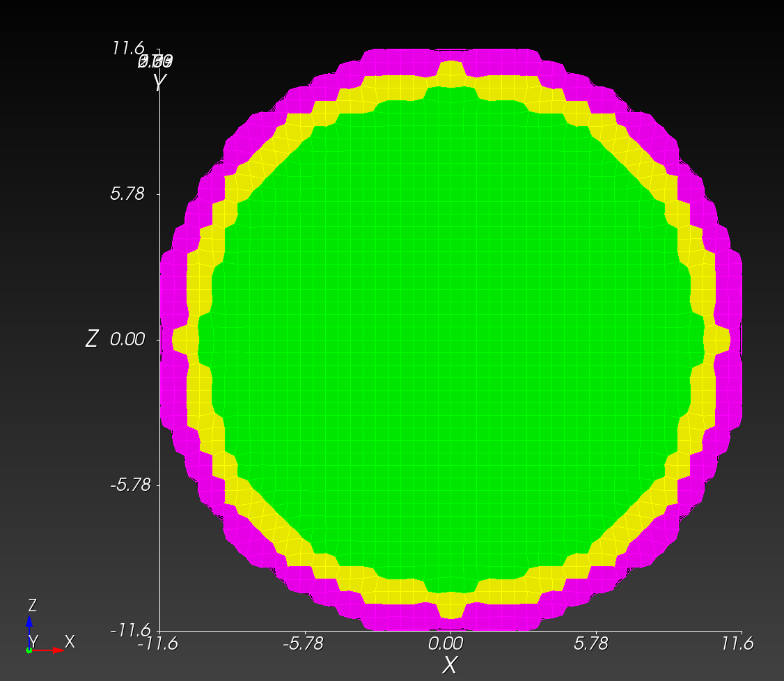 | 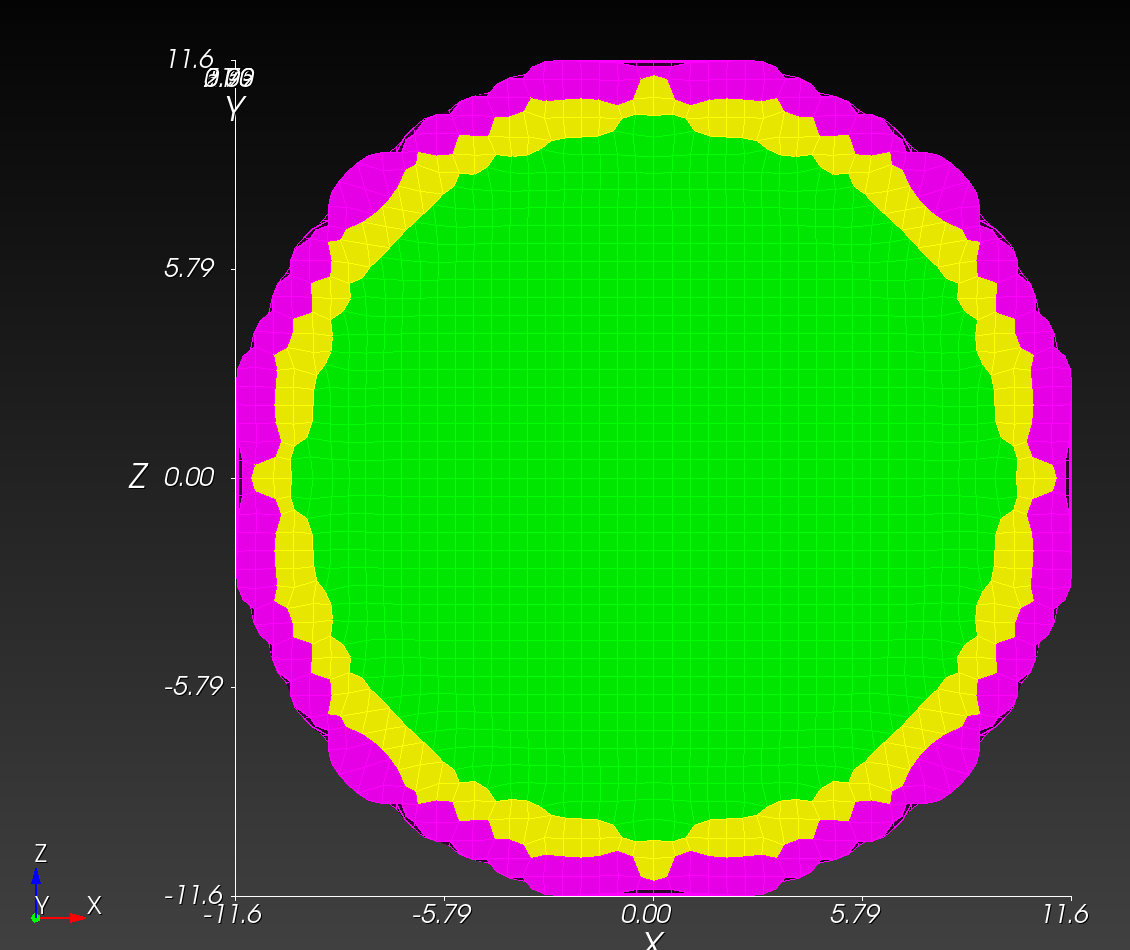 |
Smooth with various number of iterations:
automesh mesh hex \
--remove 0 \
--xscale 0.5 --yscale 0.5 --zscale 0.5 \
--xtranslate -12 --ytranslate -12 --ztranslate -12 \
--input spheres_resolution_2.npy \
--output sr2s10.exo \
smooth \
--hierarchical \
--iterations 10
automesh mesh hex \
--remove 0 \
--xscale 0.5 --yscale 0.5 --zscale 0.5 \
--xtranslate -12 --ytranslate -12 --ztranslate -12 \
--input spheres_resolution_2.npy \
--output sr2s50.exo \
smooth \
--hierarchical \
--iterations 50
Quality Metrics
Assess element quality to avoid oversmoothing:
automesh mesh hex \
--remove 0 \
--xscale 0.5 --yscale 0.5 --zscale 0.5 \
--xtranslate -12 --ytranslate -12 --ztranslate -12 \
--input spheres_resolution_2.npy \
--output sr2s10.inp \
smooth \
--hierarchical \
--iterations 10

automesh metrics \
--input sr2s10.inp \
--output sr2s10.csv
automesh mesh hex \
--xscale 0.5 --yscale 0.5 --zscale 0.5 \
--xtranslate -12 --ytranslate -12 --ztranslate -12 \
--input spheres_resolution_2.npy \
--output sr2s50.inp \
smooth \
--hierarchical \
--iterations 50

automesh metrics \
--input sr2s50.inp \
--output sr2s50.csv
With figio and
the hist_sr2sx.yml recipe,
cd ~/autotwin/automesh/book/analysis/sphere_with_shells/recipes
figio hist_sr2sx.yml
we obtain the following element quality metrics:
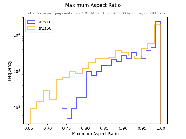
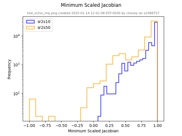
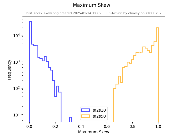
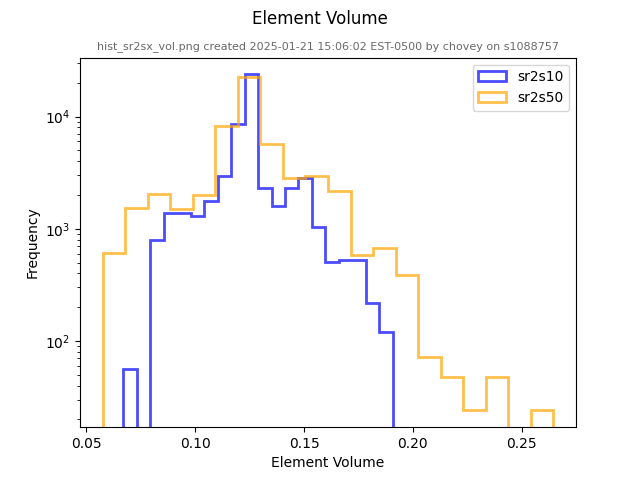
Comparisons
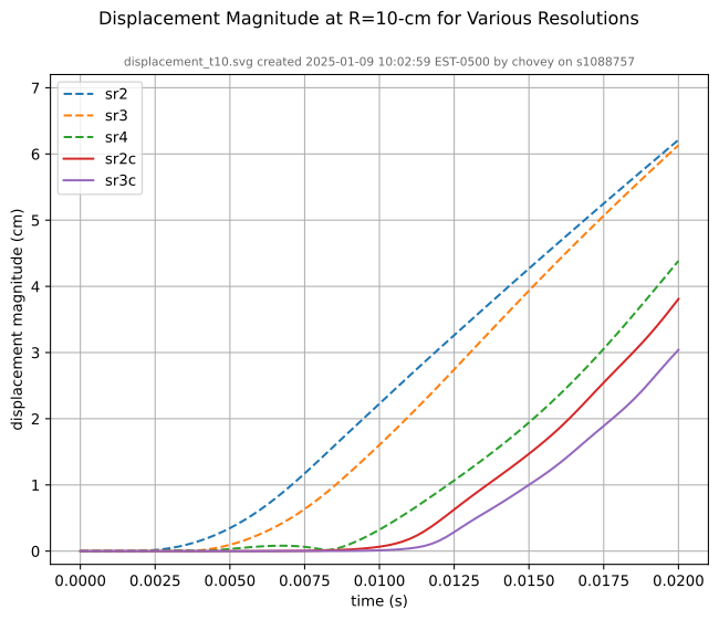
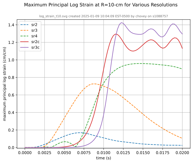
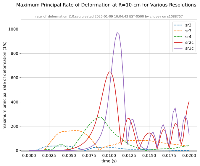
Conforming versus Segmented Meshes
We define a conforming mesh as a traditional finite element mesh that has nodal placement on the boundary of the geometry approximated by the mesh. A conforming mesh has a piecewise approximation of the curvature on the boundary.
In contrast, a segmented mesh (also known as a voxelized or "sugar-cube" mesh) is composed of voxels that approximate the boundary in a "stair-step" fashion, with nodal placement fixed on a regular, uniform grid of cube-shaped elements. A segmented mesh has a stair-step approximation of the curvature on the boundary.
The meshes from the Sphere with Shells section illustrate these two mesh types:
| conforming | segmented |
|---|---|
| |
| |
Both the conforming and segmented meshes approximate the true geometry: a sphere with concentric shells. Both approaches introduce error when used in finite element analysis in the calculation of quantities of interest, such as stress and strain.
We are interested in comparing the two methods, and quantifying what error the segmented approach introduces relative to the conforming approach.
For the spheres with shells example above, we were able to readily create two de novo meshes (the conforming mesh and the segmented mesh). There are instances, however, where a traditional, conforming finite element mesh exists, but a segmented version of the same geometry does not exist.
To create a segmented version of a conforming mesh, we created the segment command. Following are a examples using the segment functionality.
Recovering the Segmented Sphere
We use the conf_0.5cm.g file as our start point. See the Mesh Creation and Visualization section for a download link. Our objective it to recover the segmented version of the model, shown above, using the segment command.
# Clone the .g to .exo
cp conf_0.5cm.g conf_0.5cm.exo

automesh segment hex -i conf_0.5cm.exo -o conf_0.5cm_vox_segmented_g2_s0p5.exo -g 2 -s 0.5
automesh segment hex -i conf_0.5cm.exo -o conf_0.5cm_vox_segmented_g2_s0p5.inp -g 2 -s 0.5
The resulting mesh from conf_0.5cm_segmented_g2_s0p5.exo is shown (with a cut plane to show the interior) below:
| midline | isometric |
|---|---|
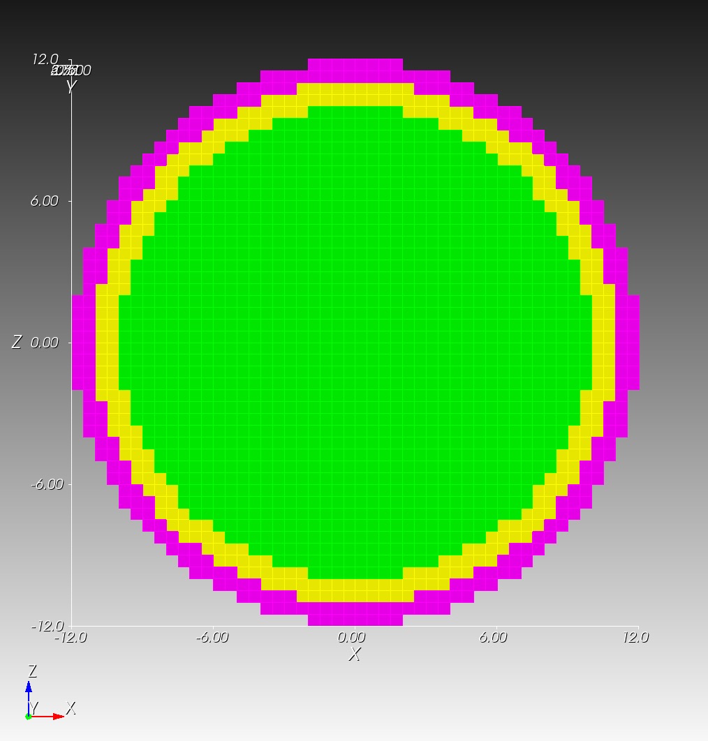 | 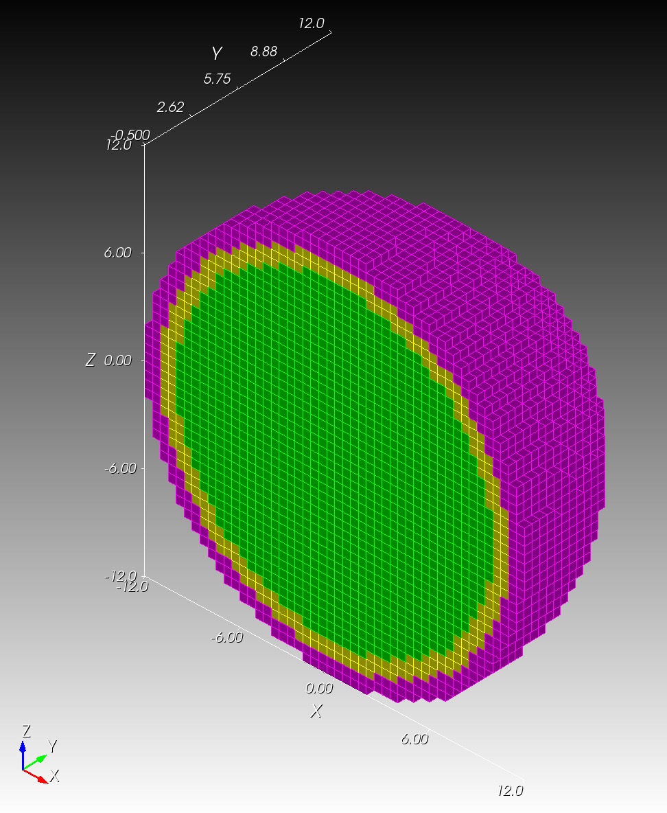 |
The conf_0.5cm_segmented_g2_s0p5.inp file mesh matches conf_0.5cm_segmented_g2_s0p5.exo exactly. Note that these new segmented meshes are slightly different from the original segmentations since they are created from a conforming mesh source.
RMU Brain Model
The RMU brain model, All_Hex_Dec, is a model of a human head.
Source Files
| file | md5 checksum | size |
|---|---|---|
All_Hex_Dec.inp | 4e376f7d551890b807cabc1d89630772 | 212 MB |
All_Hex_Dec.exo | 5df6f584a30139cb89e6e6917f843f55 | 66 MB |
test_1_1.exo | 5c0f02a7960890ffbe536493c4993104 | 95 MB |
test_1_2.exo | db674b42065cd9de9c8eb30ce2945c0f | 13 MB |
test_1_3.exo | 50da29122a0435672e62156308120ea9 | 4 MB |
test_2_1.exo | d108b4fe0aa524610fbe036e337fc6e1 | 105 MB |
test_3_0p8.exo | 60dddb70a9b018b4a25a35850c676eb6 | 205 MB |
test_3_0p8.inp | 63da6d1266a86561209ccda5f69bca23 | 541 MB |
The model has 12 blocks composing the various anatomy of the head and brain, shown below.
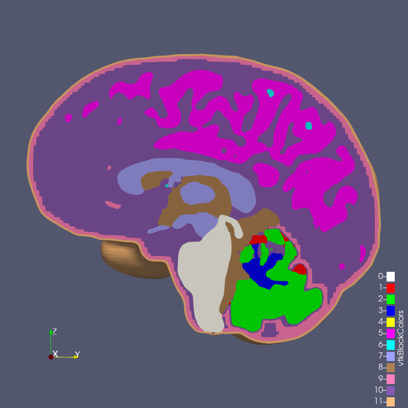
Figure 6.2-1: RMU brain model All_Hex_Dec.exo
With this conforming mesh, we create segmented meshes with the segment command, for example,
automesh segment hex --input All_Hex_Dec.exo --output test_3_0p8.exo --grid 3 --size 0.8e-3
Because All_Hex_Dec.exo and All_Hex_Dec.inp are in units of meters, we specify --size 0.8e-3 to obtain a voxel side length size of 0.8 mm.
The output files have the naming convention test_x_y.exo where
xis the grid number,yis the element length in mm,- and
0p8means0.8 mm.
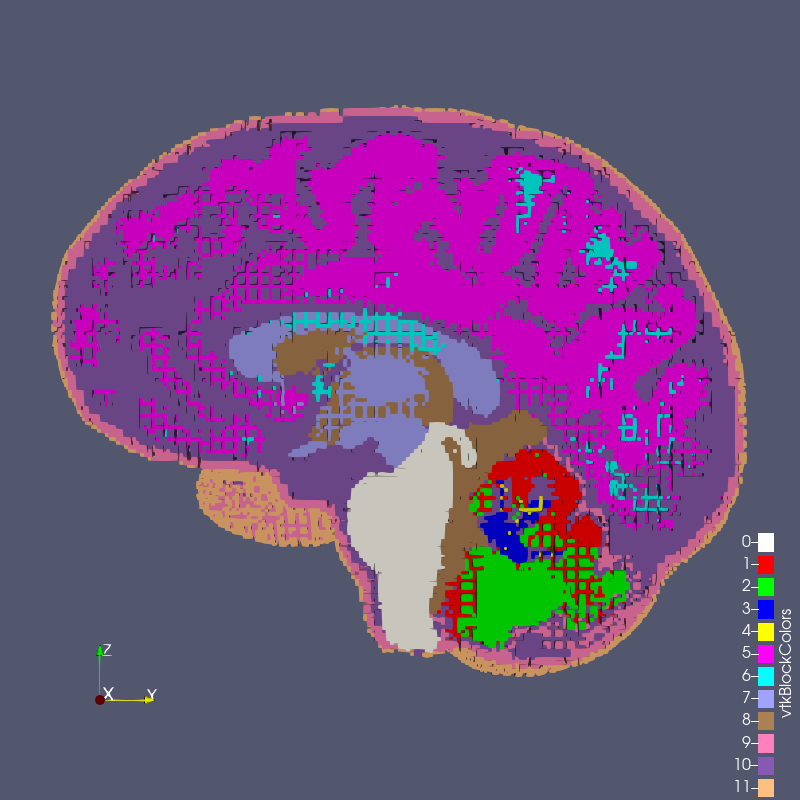
Figure 6.2-2: test_1_1.exo created with options --grid 1 --size 1

Figure 6.2-3: test_1_2.exo created with options --grid 1 --size 2

Figure 6.2-4: test_1_3.exo created with options --grid 1 --size 3
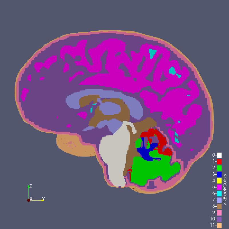
Figure 6.2-5: test_2_1.exo created with options --grid 2 --size 1
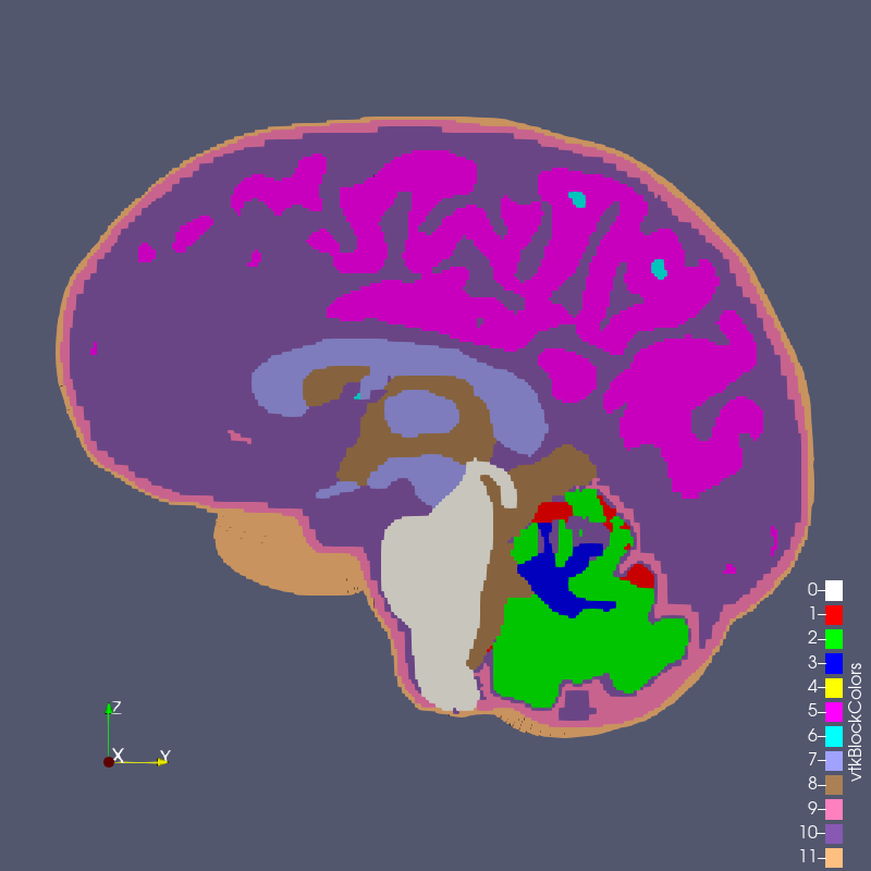
Figure 6.2-6: test_3_0p8.exo created with options --grid 3 --size 0.8
Comparison
All_Hex_Dec.exo | test_3_0p8.exo |
|---|---|
| |
Isosurfaces
Isosurfacing extracts a surface from a three-dimensional scalar field — the
step that turns a segmented volume into a triangulated boundary.
Introduction defines the problem and surveys
the three methods used in practice, including the one automesh currently
implements. Marching Cubes
and Dual Contouring cover those two
widely used general-purpose algorithms in detail.
Introduction
Isosurfacing is a method to extract the surface from a three-dimensional scalar field. A scalar field assigns a scalar value to every point in three-dimensional space. When every point in the domain sits on a regular (i.e., uniform) three-dimensional grid, the scalar field is a voxel field.
The simplest non-trivial voxel field takes only two integer values, 0
and 1. A 0 marks a point outside the field. A 1 marks a point inside
it, or on its boundary. The interface between 0 and 1 everywhere in the
grid is the field's isosurface.
Real segmentations are rarely binary. A material segmentation typically
assigns a distinct positive integer label to each material, with 0
reserved for void. The isosurface generalizes directly: it is the
interface wherever any two labels differ, not only where a label meets
void. automesh already works this way — mesh tri
produces isosurfaces of the material boundaries, plural, and the
cuberille implementation below emits a face wherever two face-adjacent
voxels' labels differ, whichever two labels they are. Any isosurfacing
method in automesh needs to preserve that: a method that only finds
the outer material/void boundary would be a regression, not an upgrade.
See Marching Cubes for how
Marching Cubes stands on this.
Three approaches, not two
Marching Cubes and Dual Contouring are the two isosurfacing algorithms
most often cited in the literature, covered in detail on the next two pages.
But a third, older approach exists, and it is the default in automesh.
Cuberille: the mesh tri default
By default, automesh mesh tri (--cubes cuberille) builds its output
surface by walking the grid once. For every pair of face-adjacent voxels
whose labels differ, the algorithm emits a quad face exactly on the voxel
boundary between them — no interpolation, no gradient information.
Each quad splits into two triangles, coincident vertices weld together, and
any resulting non-manifold "pinch" vertex is duplicated to restore a clean
2-manifold. The result is the exact voxel-boundary surface: axis-aligned,
stair-stepped, and topologically faithful to the segmentation it came from.
This is the cuberille method, first described by Herman and Liu1 in 1979 for reconstructing 3D organ surfaces from CT slices. It predates both Marching Cubes (1987) and Dual Contouring (2002).
Why it matters for mesh tri
Cuberille's stair-stepping is why cuberille output is typically smoothed
afterward — mesh tri smooth chains Laplace or Taubin smoothing directly
onto it, and mesh tri smooth remesh can follow that with remeshing. The
voxel-boundary surface is a faithful but blocky starting point. With
cuberille, smoothing, not the isosurfacing step itself, produces a
visually smooth result.
Marching Cubes and Dual Contouring take the opposite approach: both
interpolate a smoother surface during extraction, at the cost of losing
the guarantee that every output vertex sits exactly on a voxel boundary.
Marching Cubes interpolates along voxel edges. Dual
Contouring places a vertex inside each voxel, using
gradient information to better preserve sharp features. Marching Cubes is
available through mesh tri --cubes marching. automesh does not implement
Dual Contouring.
References
-
Herman GT, Liu HK. Three-dimensional display of human organs from computed tomograms. Computer Graphics and Image Processing. 1979;9(1):1-21. link ↩
Marching Cubes
Marching Cubes, originally proposed by Lorensen and Cline in 19871,
operates on each voxel in the 3D grid on an independent basis.
For each voxel, the eight nodes of the voxel are evaluated as outside (0) the scalar field or inside (1) the scalar field. The eight nodes, classified as either 0 or 1, create 256 () possible configurations. Of these combinations, only 15 are unique configurations, after symmetry and rotation considerations. For each configuration, Marching Cubes generates a set of triangles to approximate the isosurface.
Ambiguous Cases
Some configurations of the original table have more than one valid triangulation. An example is a cube face with two diagonal nodes inside and two outside. The original table picks one triangulation per configuration. Two cubes that share such a face can then pick incompatible triangulations. The result is a crack, or an edge shared by more than two triangles.
Manifold: "The mesh forms a 2D manifold if the local topology is everywhere equivalent to a disc; that is, if the neighborhood of every feature consists of a connected ring of polygons forming a single surface (see Figure 2 of Luebke2 reproduced below). In a triangulated mesh displaying manifold topology, exactly two triangles share every edge, and every triangle shares an edge with exactly three neighboring triangles. A 2D manifold with boundary permits boundary edges, which belong to only one triangle."
| manifold | non-manifold |
|---|---|
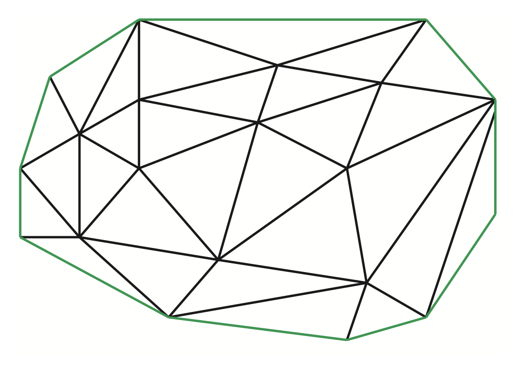 | 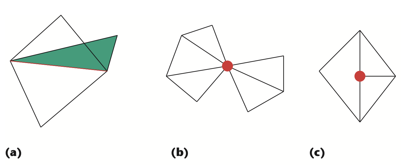 |
Figure 7.2-1: Reproduction of Luebke2 Figure 2 (left) showing a manifold mesh, and Figure 3 (right) showing a non-manifold mesh because of (a) an edge shared by more than two triangles, (b) a vertex shared by two unconnected sets of triangles, and (c) a T-junction vertex.
Lewiner et al.3 resolve the ambiguous cases.
Their algorithm adds the missing cases to the original table.
It picks each triangulation so that two cubes sharing a face agree on that face.
This removes the cracks that the original table can produce.
automesh uses this variant.
A binary field needs one further caution.
It takes only the values 0 and 1, so the level 0.5 equals the field value at the saddle of an ambiguous face.
At such a tie, the Lewiner method can leave an edge shared by more than two triangles.
The tie arises only where the segmentation contains an ambiguous configuration.
The unit sphere does not create this pathology.
Marching Cubes in automesh
mesh tri --cubes marching extracts the surface of each material separately.
automesh builds the scalar field from the segmentation, one material at a time:
- The field is
1.0at every voxel of the material and0.0elsewhere. - A one-voxel border of
0.0surrounds the field, so the surface closes at the edge of the grid. - The surface sits where the field equals
0.5, halfway between0and1. - Every grid edge that the surface crosses runs from a
0to a1, so the surface crosses it at its midpoint. Every output vertex therefore sits at the midpoint of a grid edge. - Degenerate triangles are not output.
mesh hex --marching and --inflate use the same extraction on a uniform lattice cut by a tessellation.
Advantages
- Simple implementation; uses only interpolation between voxel corners.
- Interpolates along edges between voxel corners. With a continuous scalar field, this gives a smooth surface. This can be an advantage when smooth meshes are desired but is a disadvantage when sharp edges are desired.
- With the Lewiner variant, the ambiguous cases do not produce cracks or inconsistent triangulations.
Disadvantages
- The surface is only as smooth as the scalar field.
automeshsupplies a binary field, so the interpolation puts every vertex at an edge midpoint. The surface is a chamfered version of the voxel staircase, not a smooth surface.mesh tri smoothremoves more of it. - It cannot place a vertex inside a voxel, so it does not preserve sharp features. Dual Contouring does.
Multi-material interfaces
automesh runs Marching Cubes once per material, and each run extracts that material's boundary independently.
Each material gets its own block of triangles.
Two adjacent materials each carry a copy of their shared interface.
The two copies coincide in position, and they are separate nodes, so the mesh is not merged across the interface.
Wu and Sullivan4 classify each cube by the set of labels that touch it. Frisken5 extends the Dual Contouring family the same way. Either would be the reference for a multi-label method.
References
-
Lorensen WF. Marching cubes: A high resolution 3D surface construction algorithm. Computer Graphics. 1987;21. link ↩
-
Luebke DP. A developer's survey of polygonal simplification algorithms. IEEE Computer Graphics and Applications. 2001 May;21(3):24-35. link ↩ ↩2
-
Lewiner T, Lopes H, Vieira AW, Tavares G. Efficient implementation of Marching Cubes' cases with topological guarantees. Journal of Graphics Tools. 2003;8(2):1-15. link ↩
-
Wu Z, Sullivan JM Jr. Multiple material marching cubes algorithm. International Journal for Numerical Methods in Engineering. 2003;58(2):189-207. link ↩
-
Frisken SF. SurfaceNets for multi-label segmentations with preservation of sharp boundaries. Journal of Computer Graphics Techniques. 2022;11(1):34-54. link ↩
Dual Contouring
Dual Contouring (DC) was originally proposed by Ju et al.1 in 2002.
DC improves upon the Marching Cubes algorithm. DC uses the dual grid of the voxel data, locating nodes of the surface within the voxel, rather than on the edge of the voxel (as done with Marching Cubes).
Boris2 created a figure, reproduced below, that illustrates the differences between Marching Cubes and DC.
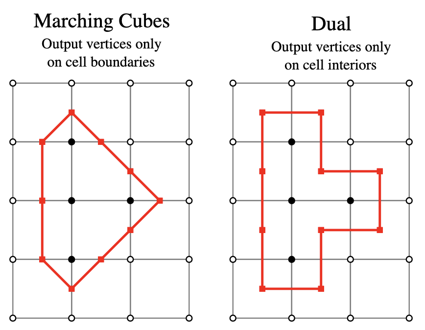
Figure 7.3-1: Reproduction of the figure from Boris2, illustrating, in two dimensions, the differences between Marching Cubes and DC. White circle are outside points. Black circles are inside points. In Marching Cubes, the red points indicate surface vertices at edge intersections. In DC, the red points indicate surface vertices within a voxel.
Advantages
- "[C]an produce sharp features by inserting vertices anywhere inside the grid cube, as opposed to the Marching Cubes (MC) algorithm that can insert vertices only on grid edges."3
Disadvantages
- More complicated than Marching Cubes since DC uses both position and normal (gradient) information at voxel edges to locate the surface intersection.
- "...unable to guarantee 2-manifold and watertight meshes due to the fact that it produces only one vertex for each grid cube." "DC is that it does not guarantee 2-manifold and intersection-free surfaces. A polygonal mesh is considered as being 2-manifold if each edge of the mesh is shared by only two faces, and if the neighborhood of each vertex of the mesh is the topological equivalent of a disk." 3
References
-
Ju T, Losasso F, Schaefer S, Warren J. Dual contouring of hermite data. In Proceedings of the 29th annual conference on Computer graphics and interactive techniques 2002 Jul 1 (pp. 339-346). link ↩
-
Boris. Dual Contouring Tutorial. Available from: https://www.boristhebrave.com/2018/04/15/dual-contouring-tutorial/ [Accessed 18 Jan 2025]. link ↩ ↩2
-
Rashid T, Sultana S, Audette MA. Watertight and 2-manifold surface meshes using dual contouring with tetrahedral decomposition of grid cubes. Procedia engineering. 2016 Jan 1;163:136-48. link ↩ ↩2
Subdivision
Surface subdivision is a geometric modeling technique that defines smooth curves or surfaces as the limit of a sequence of successive refinements.
Developed as a generalization of spline surfaces, subdivision allows for the representation of complex, arbitrary control meshes while avoiding the topological constraints and "cracking" issues often associated with traditional Non-Uniform Rational B-Splines (NURBS).
Various algorithms have been established to handle different mesh types and desired continuity:
- The Catmull-Clark scheme is frequently used for quadrilateral meshes to produce continuous surfaces, while
- The Loop subdivision scheme is a popular approximating method specifically designed for triangular meshes.
By iteratively applying simple refinement rules—typically involving a "splitting" step to increase resolution and an "averaging" step to relocate vertices—subdivision transforms a coarse initial shape into a highly detailed, smooth limit surface suitable for high-end animation and scalable rendering.
Octa Loop
This example uses Loop subdivision to transform an octahedron into a sphere. The results below are based on Octa-Loop Subdivision Scheme (GitHub).
We create a unit radius octahedron template, and successively refine it into a sphere. The sphere is a useful baseline subject of study because it:
- Can easily be approximated by a voxel stack at various resolutions,
- Can easily be approximated by a finite element mesh,
- Has a known analytic volume, and
- Has a known analytic local curvature.
Base Octahedron
We created a unit radius template, octa_base.obj, with contents listed below:
v 1.0 0.0 0.0
v 0.0 1.0 0.0
v -1.0 0.0 0.0
v 0.0 -1.0 0.0
v 0.0 0.0 1.0
v 0.0 0.0 -1.0
f 1 2 5
f 2 3 5
f 3 4 5
f 4 1 5
f 2 1 6
f 3 2 6
f 4 3 6
f 1 4 6
Refinement
The refinement below was created with MeshLab 2022.02, Subdivision Surfaces LS3 Loop, based on Boye et al.1
| name | image | file size |
|---|---|---|
octa_loop00.stl | 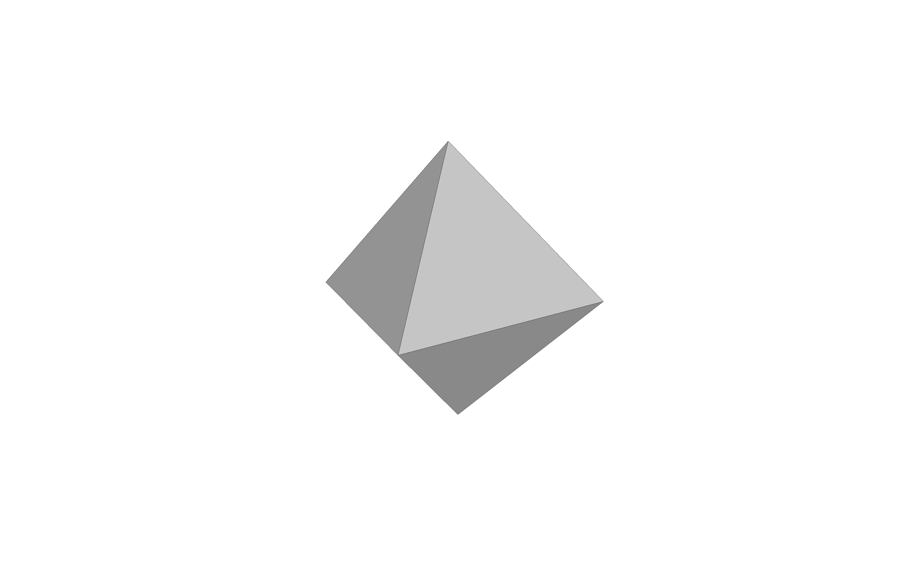 | 2.1kB |
octa_loop01.stl | 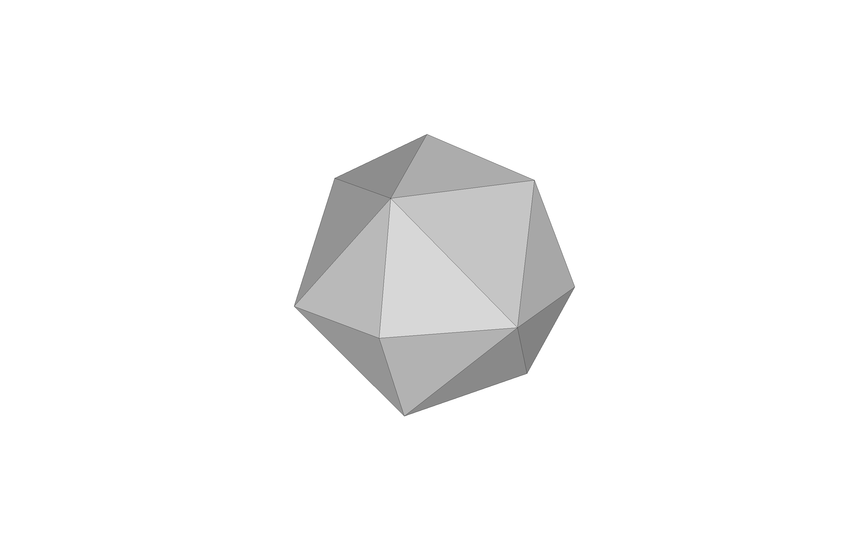 | 8.3kB |
octa_loop02.stl G | 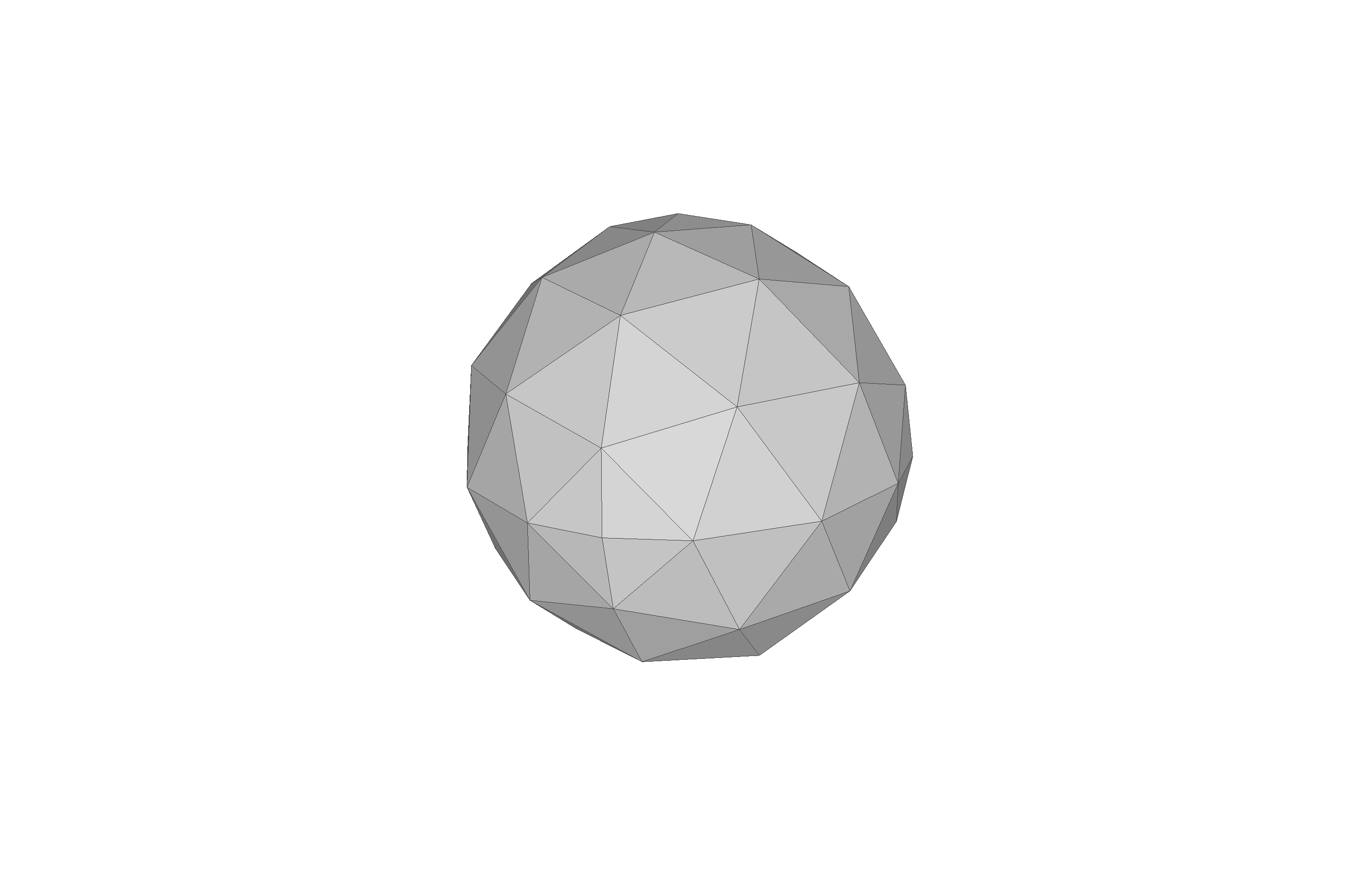 | 33kB |
octa_loop03.stl G | 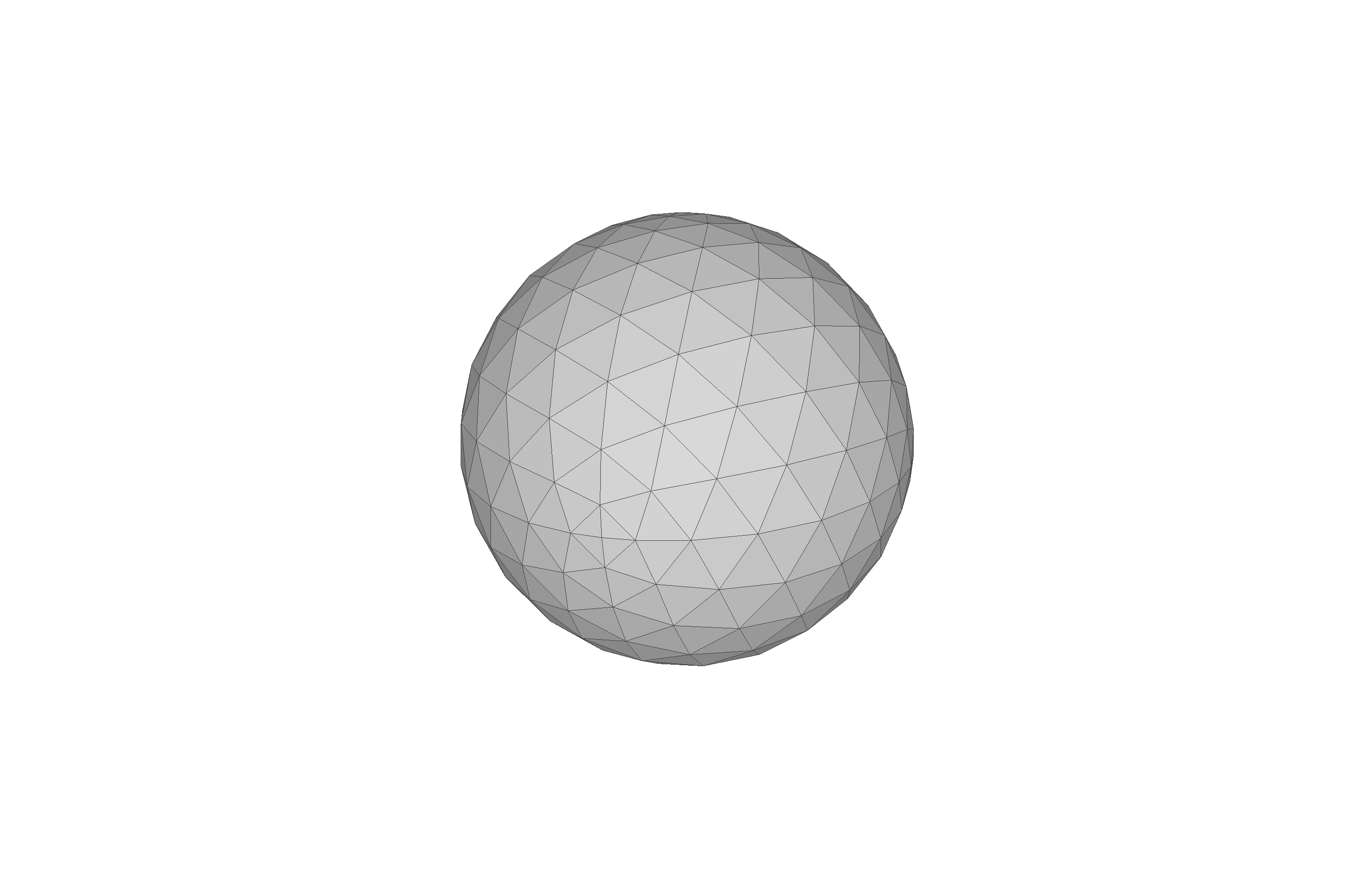 | 132kB |
octa_loop04.stl G | 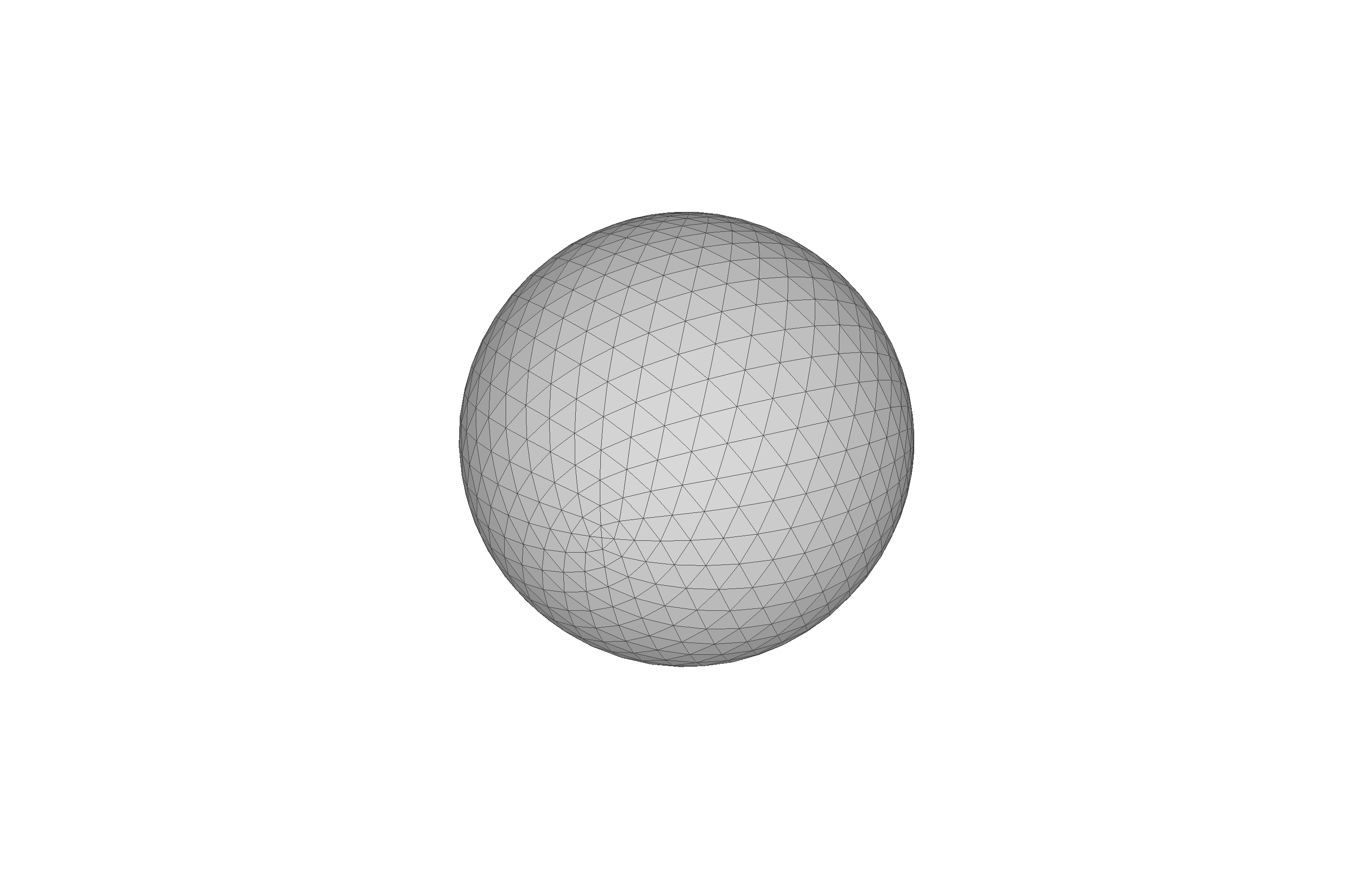 | 526kB |
octa_loop05.stl G | 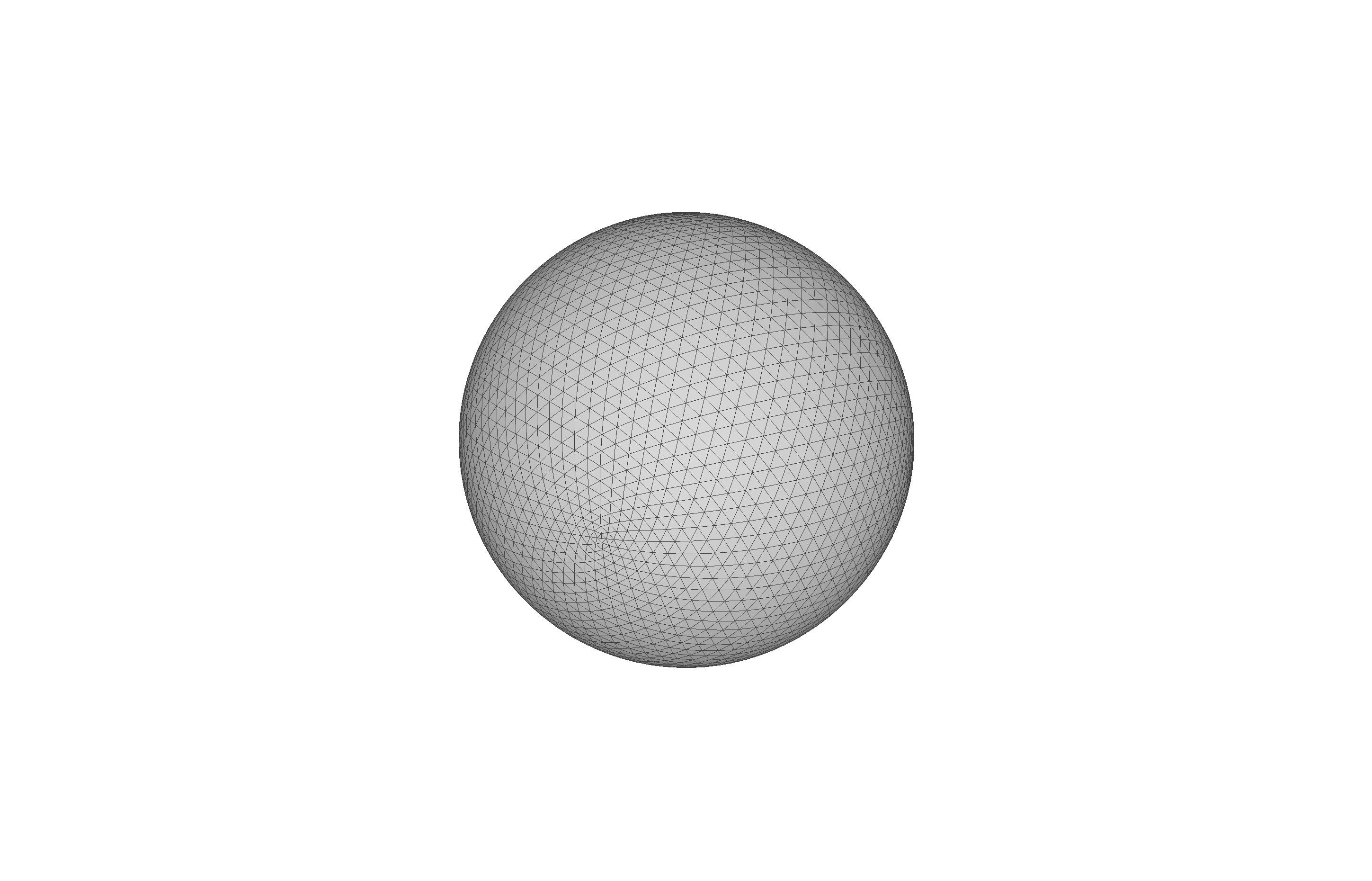 | 2.1MB |
octa_loop06.stl G | 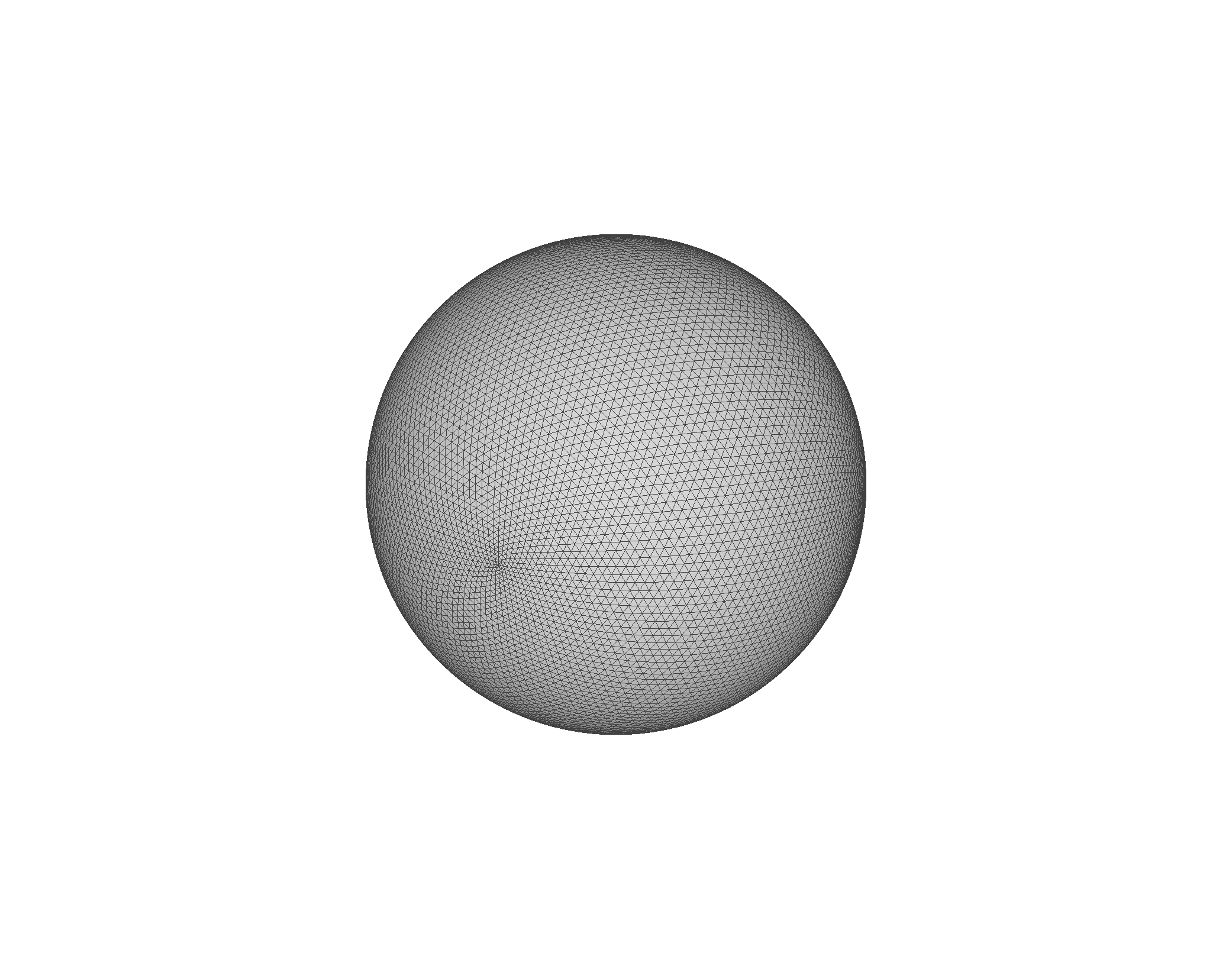 | 8.6MB |
octa_loop07.stl G | 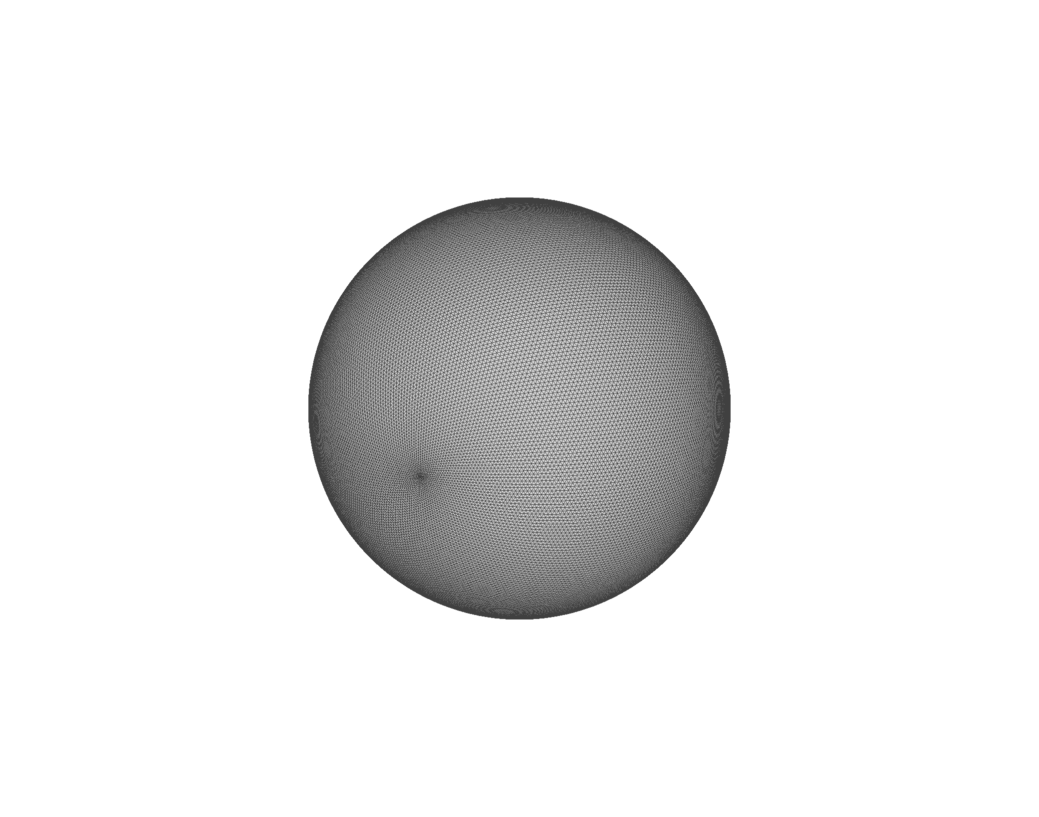 | 33MB |
Items with
Gare not on the repository; they are on Google Drive because of their large file size.
Geometric Metrics
- The surface area of a sphere is , and when , .
- The volume of a sphere is , and when , .
Using the Euler Characteristic for a sphere (), we can verify the progression from the base octahedron ():
| Iteration () | Vertices () | Edges () | Faces () | Calculation () |
|---|---|---|---|---|
| 0 (Base) | 6 | 12 | 8 | 6+12=18 |
| 1 | 18 | 48 | 32 | 18+48=66 |
| 2 | 66 | 192 | 128 | 66+192=258 |
| 3 | 258 | 768 | 512 | 258+768=1,026 |
| 4 | 1,026 | 3,072 | 2,048 | 1,026+3,072=4,098 |
| 5 | 4,098 | 12,288 | 8,192 | 4,098+12,288=16,386 |
| 6 | 16,386 | 49,152 | 32,768 | 16,386+49,152=65,538 |
| 7 | 65,538 | 196,608 | 131,072 | 65,538+196,608=262,146 |
The recursive relationships for a closed triangular mesh:
- Faces:
- Edges:
- Vertices:
Sculpt Baseline
We created Sculpt baseline meshes with the sculpt_stl_to_inp.py script as
(atmeshenv) ~/autotwin/mesh/src/atmesh> python sculpt_stl_to_inp.py
and create standard views in Cubit with
Cubit>
graphics perspective off  # orthogonal, not perspective view
up 0 0 1  # z-axis points up
view iso # isometric x, y, z camera
quality volume 1 scaled jacobian global draw histogram draw mesh list
to produce the following results:
| iter | image | cells | nodes nnp | elements nel | element density nel |
|---|---|---|---|---|---|
| 0 | 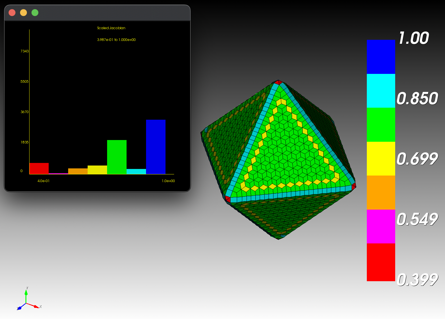 | 35x35x35 | 8,696 | 7,343 | 5,507 |
| 1 | 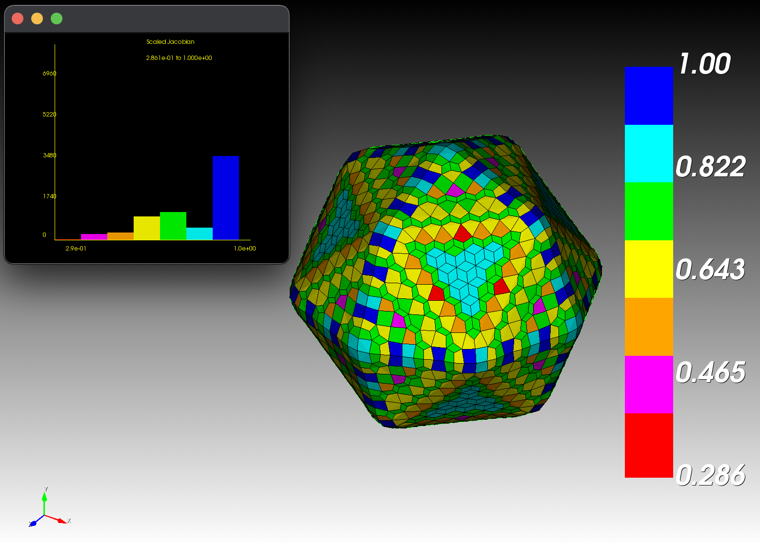 | 28x28x28 | 8,133 | 6,960 | 2,365 |
| 2 | 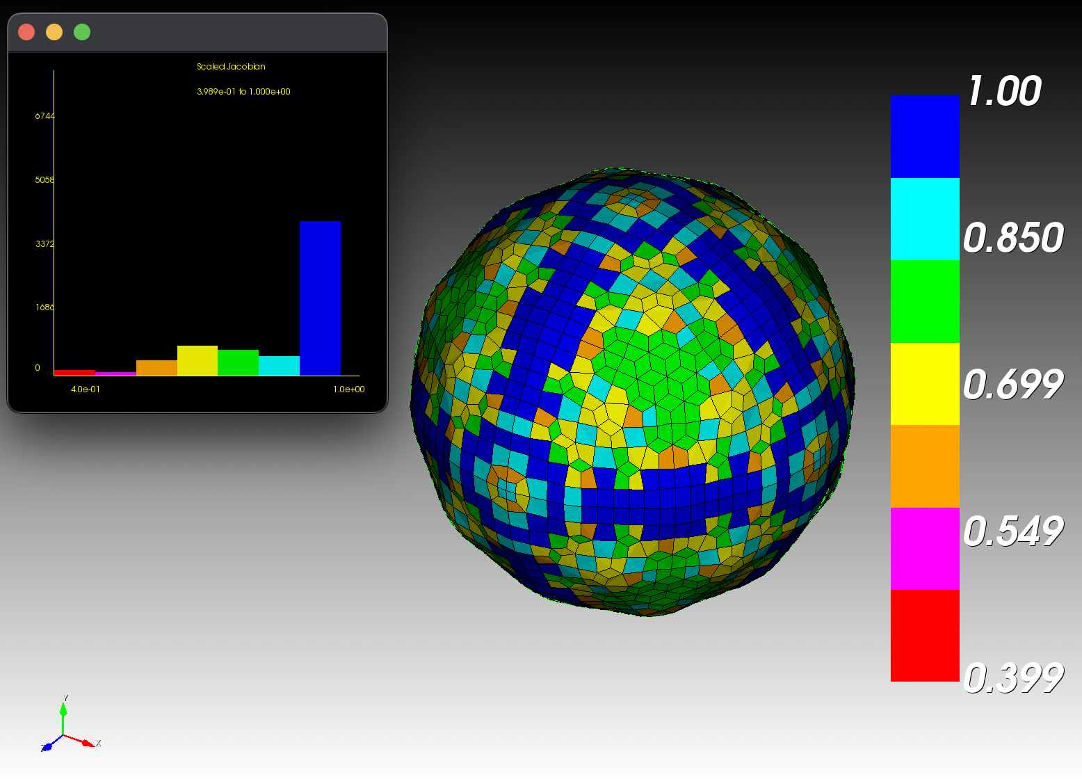 | 26x26x26 | 7,833 | 6,744 | 1,762 |
| 3 | 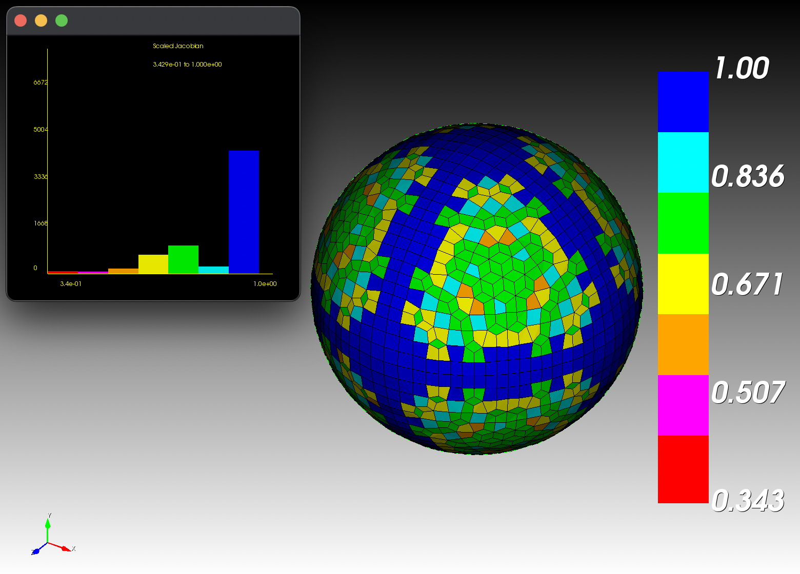 | 26x26x26 | 7,731 | 6,672 | 1,630 |
| 4 | 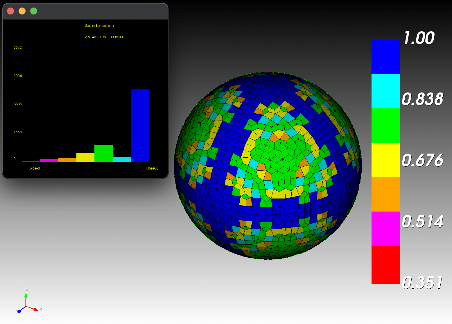 | 26x26x26 | 7,731 | 6,672 | 1,600 |
| 5 | 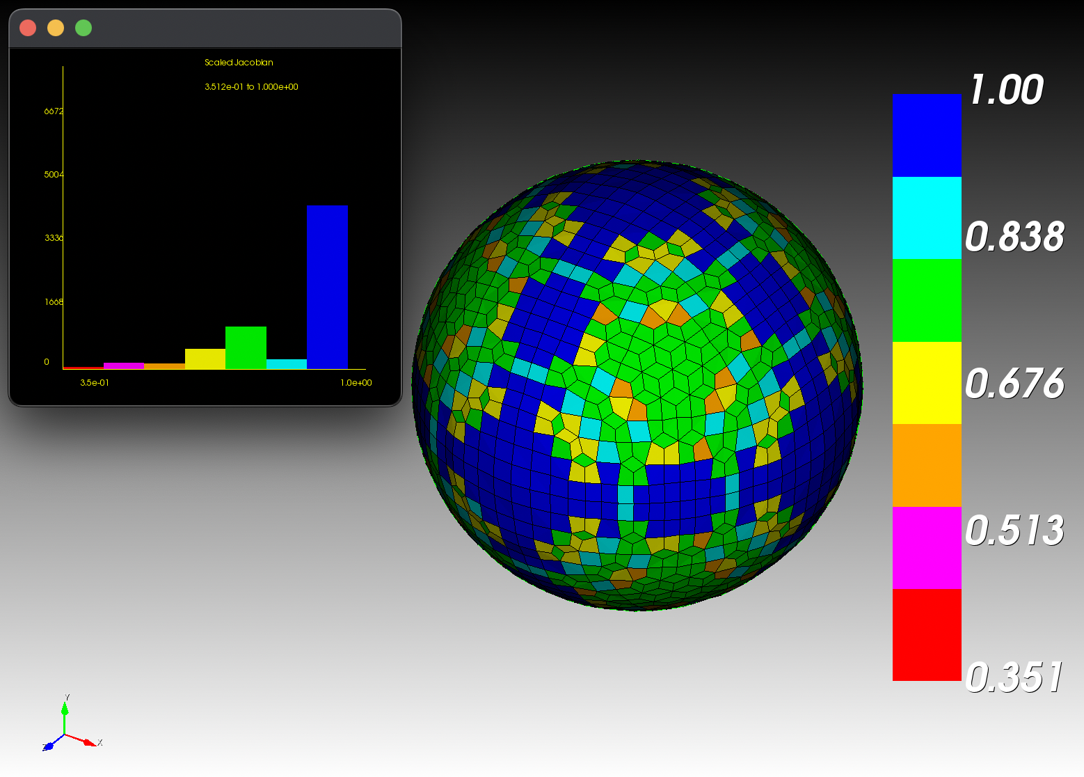 | 26x26x26 | 7,731 | 6,672 | 1,596 |
| 6 | 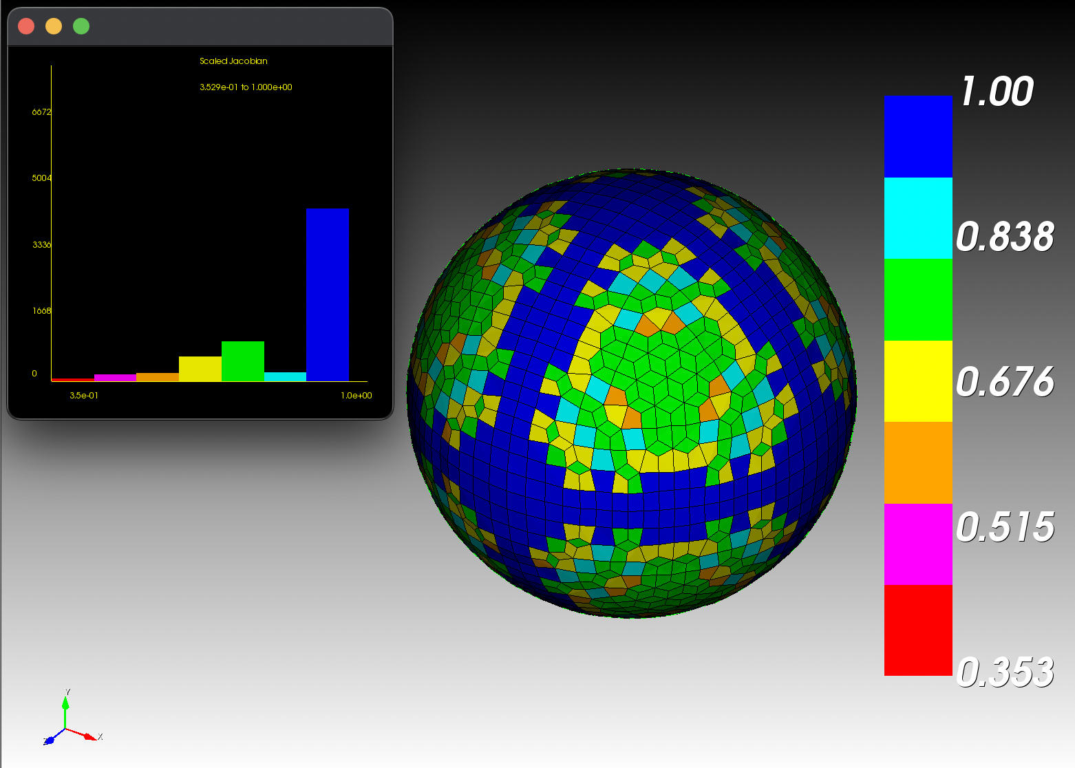 | 26x26x26 | 7,731 | 6,672 | 1,595 |
| 7 | 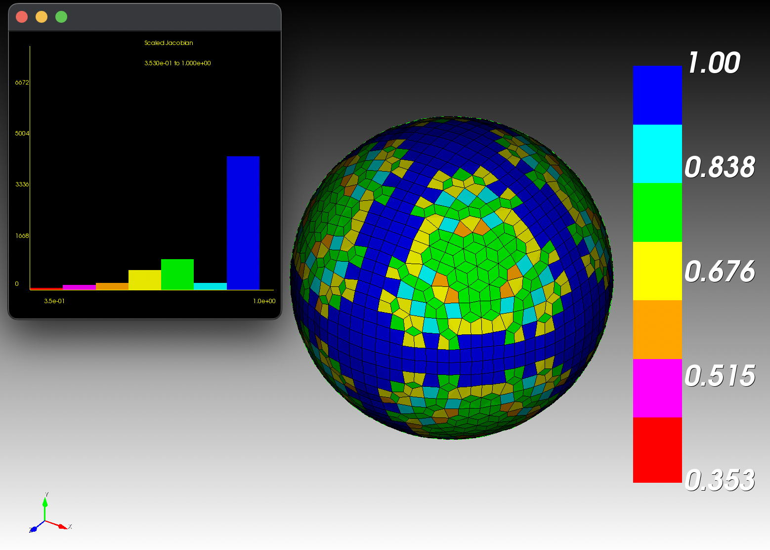 | 26x26x26 | 7,731 | 6,672 | 1,595 |
References
- Octa-Loop Subdivision Scheme (GitHub)
- Documentation detailing the Octa-Loop scheme, a variant of Loop subdivision optimized for octahedrally refined meshes.
- Subdivision Surfaces Lecture Notes (Stanford University)
- A comprehensive academic overview of subdivision concepts, including the mathematical foundations of the Catmull-Clark and Loop schemes.
- Stanford cs468-10-fall Subdivision http://graphics.stanford.edu/courses/cs468-10-fall/LectureSlides/10_Subdivision.pdf and Google Drive repo copy
- Catmull–Clark Subdivision Surface (Rosetta Code)
- A technical resource providing algorithmic steps and multi-language code implementations for the Catmull-Clark subdivision process.
- Recursively Generated B-Spline Surfaces (Original Paper)
- The seminal 1978 paper by Edwin Catmull and James Clark that introduced the method for generating smooth surfaces from arbitrary topological meshes (referenced within the other materials).
- Catmull, E., & Clark, J. (1978). Recursively generated B-spline surfaces on arbitrary topological meshes. Computer-Aided Design, 10(6), 350-355. https://doi.org/10.1016/0010-4485(78)90110-0
- Loop, C. (1987). Smooth subdivision surfaces based on triangles [Master's thesis, University of Utah]. https://www.microsoft.com/en-us/research/wp-content/uploads/2016/02/thesis-1.pdf
- https://docs.juliahub.com/Meshes/FuRcu/0.17.1/algorithms/refinement.html#Catmull-Clark
-
Boyé S, Guennebaud G, Schlick C. Least squares subdivision surfaces. In Computer Graphics Forum 2010 Sep (Vol. 29, No. 7, pp. 2021-2028). Oxford, UK: Blackwell Publishing Ltd. ↩
Hexahedral Meshing from a Surface
Given a closed, manifold, triangular surface — an stl tessellation, for example — automesh produces an all-hexahedral volume mesh of the region the surface encloses. This page describes the algorithm end to end.
automesh mesh hex --input surface.stl --output mesh.exo --scale 8
The method is a dual method: Rather than fitting hexahedra to the surface directly, it builds an octree over the enclosed volume and constructs the dual of that octree. The dual of a balanced octree is all-hexahedral by construction, which guarantees the output mesh to consist of only hexahedral elements.
Two Meshes, Two Vocabularies
Because a dual method involves two distinct meshes at once, it is worth fixing terminology before describing the algorithm. Throughout this page:
- A cell is a box of the octree — the primal structure. A leaf cell is one that has not been subdivided further. Cells are what the octree refines, balances, and pairs.
- A hexahedron, or element, belongs to the dual mesh — the output. Hexahedra are what the finished mesh is made of, and what quality metrics are computed on.
The two are related by the dual correspondence, which inverts dimension:
| Octree (primal) | Dual mesh (output) |
|---|---|
| leaf cell | node, at the cell center |
| vertex where cells meet | hexahedron, joining those cells' center nodes |
So a dual node sits at the center of each octree leaf cell, and a dual hexahedron is formed around each octree vertex, joining the centers of the eight leaf cells meeting there. Where the octree is uniform, this is exactly eight equal cells meeting at a corner and the resulting hexahedron is a perfect cube. Where the octree changes level, fewer or unequal cells meet, and a template supplies the connectivity instead — the subject of Dualization.
The pipeline has five stages, and stage 3 is the pivot between the two vocabularies: everything upstream of it operates on octree cells, and everything downstream operates on dual hexahedra.
| Stage | Operates on | |
|---|---|---|
| 1 | Octree construction from the shape diameter function | cells |
| 2 | Equilibration, which balances and pairs the octree | cells |
| 3 | Dualization, which converts cells into hexahedra via templates | cells → hexahedra |
| 4 | Trimming, which discards hexahedra lying outside the surface | hexahedra |
| 5 | Buffering, which fits the boundary to the surface | hexahedra |
Stage 3 consumes the octree and emits the dual mesh. The octree plays no further role once dualization is complete — trimming and buffering never consult it, and never subdivide, coarsen, or otherwise revisit a cell. Whatever the templates produced is what the remaining stages must work with, which is why the interior quality bound established at stage 3 survives to the finished mesh.
Cutting the pipeline the other way: stages 1–3 produce the interior of the mesh and are purely combinatorial, so their quality is bounded in advance (see Template Quality). Stages 4–5 fit that interior to the actual geometry, and are the only stages that can degrade quality.
The input surface is not validated.
automeshperforms no up-front check for holes, non-manifold edges, or inconsistent orientation. A defective surface will either produce a poor mesh or fail late, during buffering, with anon-manifold boundaryerror. Verify the surface before meshing.
Consider
--strongfor quality-critical work. The balancing rule chosen during equilibration determines the guaranteed interior mesh quality. The default is weak balancing; passing--strongraises the guaranteed minimum scaled Jacobian of every interior element from to , at the cost of a larger mesh. See Balancing.
Template Quality
Because the interior is assembled exclusively from a finite catalog of templates, its quality is bounded below by construction, before any smoothing is applied. The catalogs below were measured directly from the dualization stage.
Under strong balancing, the catalog admits ten distinct values of the minimum scaled Jacobian:
| Minimum scaled Jacobian | Closed form |
|---|---|
| 0.258199 | |
| 0.402015 | |
| 0.438562 | |
| 0.447214 | |
| 0.548202 | |
| 0.577350 | |
| 0.727273 | |
| 0.894427 | |
| 0.904534 | |
| 1.000000 | cube |
The interior quality lower bound under strong balancing is therefore
Under weak balancing — the default in automesh — two additional configurations become reachable, both below :
| Minimum scaled Jacobian | Closed form |
|---|---|
| 0.246183 | |
| 0.257130 |
relaxing the lower bound to
These two configurations arise only on topologically complex inputs. Simple convex shapes such as a sphere attain under either balancing rule, so the difference between the two bounds becomes visible only on demanding geometry.
The difference has a structural explanation. Weak balancing admits a fifth edge template that strong balancing rules out; the four-template set under --strong is exactly the set illustrated in Dualization. The measured catalogs and the template inventory agree: the extra template, and the two extra quality values, appear together.
Two practical consequences follow.
Any element below the lower bound came from the boundary. Trimming and buffering are the only stages that deform geometry, so sub-bound quality in a finished mesh is always attributable to them. The interior is never the culprit, and no amount of octree refinement will fix a boundary problem.
The bound is a choice, not a constant. Passing --strong removes the two sub- configurations from the catalog outright. This is the only control automesh currently offers over interior quality — nothing downstream optimizes it — so it is worth setting deliberately rather than accepting the default.
Quality Assessment and Improvement
Element quality is reported with --metrics, which writes maximum edge ratio, minimum scaled Jacobian, maximum skew, and element volume per element:
automesh mesh hex --input surface.stl --output mesh.exo --scale 8 --metrics quality.csv
Quality can be improved after meshing with Taubin or Laplace smoothing:
automesh mesh hex --input surface.stl --output mesh.exo --scale 8 smooth --method Taubin
Taubin smoothing is preferred over Laplace, which shrinks the mesh; see Smoothing.
Optimization-based quality improvement — in particular BFGS-driven untangling and quality maximization, as described by Protais et al.1 — is the intended direction for automesh but is not yet implemented. At present, no stage of the pipeline optimizes element quality; the interior relies on the template bound, and the boundary on smoothing.
Choosing a Scale
Quality does not improve monotonically with --scale. Raising it refines the octree, which improves the resolution of the surface, but also produces more transition regions and more buffer elements — and past a point the latter dominates.
For the remeshed unit sphere sphere_n10.stl, sweeping --scale gives:
--scale | Elements | Minimum scaled Jacobian |
|---|---|---|
| 3 (default) | 7 | 0.531 |
| 4 | 37 | 0.215 |
| 5 | 73 | 0.171 |
| 6 | 183 | 0.058 |
| 7 | 235 | 0.058 |
| 8 | 393 | 0.280 |
| 9 | 551 | 0.009 |
| 10 | 804 | −0.165 |
Scale 8 is the sweet spot here; scale 10 produces inverted elements. The practical guidance is to sweep --scale and inspect --metrics rather than assuming that a larger value is better. The optimum is model-specific.
Note what the default produces: at --scale 3, this sphere yields 7 elements — enough to confirm the pipeline runs, but far too coarse to be a usable mesh. The default is a conservative starting point, not a recommendation. Expect to raise it for any real model.
--scale is a floating-point argument, so intermediate values such as --scale 7.5 are permitted; the sweep above uses integers only for legibility.
Failure Modes
non-manifold boundary. Raised during buffering. Frequent causes:
- Smoothed input tessellations. Dualizing a Taubin-smoothed surface reliably triggers this error. Smooth the hexahedral mesh after meshing, not the surface before it.
- Surfaces with holes, or self-intersections. The Stanford bunny
stanford_bunny.stlfails at every scale for this reason, even though its octree dualizes without complaint.
Degenerate or inverted elements. A minimum scaled Jacobian at or below zero indicates elements produced by the buffer layer that could not be fitted. Causes:
- Thin shells. The method fills an enclosed volume. A one-element-thick shell has almost no interior, so nearly every element is a buffer element and the template bound does not apply.
- Excessive
--scale, as shown above.
A far denser mesh than expected. Refinement is driven by local thickness, so an unintentionally thin feature — a sliver, a near-degenerate facet, a self-intersection that reads as thin — is resolved at cells across its own small thickness, and the balancing rules then propagate some of that refinement into its neighborhood. Inspect the model for unintended thin features, or coarsen --scale.
References
See also Hexahedral Metrics for the definition of the minimum scaled Jacobian.
-
Protais F, Cherchi G, Livesu M. Versatile Volume Fitting with Automatic Feature Preservation. 2026. HAL open archive, inria.hal.science. paper ↩
Octree Construction
Stage 1 of five. Operates on cells. See Hexahedral Meshing from a Surface for the pipeline overview and terminology.
The octree is sized from the shape diameter function (SDF) of the tessellation, a per-facet estimate of the local thickness of the solid, obtained by casting rays inward from each facet and measuring the distance to the opposite side.
Let denote the --scale argument, the smallest positive shape diameter — the thinnest part of the model — and the largest extent of the surface bounding box. Then the finest cell size and the maximum tree depth are
Each symbol has a direct physical reading:
| Symbol | Is | Measured in |
|---|---|---|
| thickness of the thinnest part of the solid | length | |
| edge length of the root cell, which encloses the model | length | |
| edge length of the smallest cell the tree may create | length | |
| how many cells are placed across the local thickness | count | |
| how many times the root may be halved to reach | count |
The one to build intuition on is . Rearranging gives : the thinnest feature is spanned by exactly cells. And because the octree stops subdividing a cell once it is no larger than the local thickness divided by , this holds throughout the model, not just at its thinnest point.
--scaleis the number of cells placed through the thickness of the solid. At--scale 4, a thin plate gets four cells through its thickness, and so does a thick block through its own.
and then follow as bookkeeping: is the resolution the thinnest feature demands, and is the depth needed to reach that resolution from a root cell of size , since halving times gives .
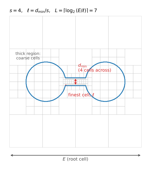
The figure shows a 2D quadtree analogue at for a dumbbell — two thick lobes joined by a thin bar. Note that the fine cells appear only along the thin bar; the lobes are meshed coarsely, because four cells across their thickness is a much larger cell. The red square is the finest cell , sized by at the bar.
Three consequences are worth stating plainly:
--scaleis not a tree depth. It is a divisor on local thickness. Because depth enters logarithmically, doubling--scaleadds approximately one level of refinement, not twice as many.- Refinement is local, not global. A thin feature is refined finely; thick regions elsewhere are not. A sliver raises the depth budget , but only cells near the sliver actually descend to it.
- Refinement is surface-driven. Cells are subdivided only where they straddle the surface. The deep interior of a thick region stays coarse regardless of .
The default is --scale 3, which is deliberately coarse. Meshes of any detail generally require considerably more; see Choosing a Scale.
Next: Equilibration, which balances and pairs the octree this stage produced.
Equilibration
Stage 2 of five. Operates on cells. See Hexahedral Meshing from a Surface for the pipeline overview and terminology.
Two conditions must hold before the octree can be dualized: the tree must be balanced, and its transition regions must be paired.
Balancing
Balancing limits the depth difference between neighboring cells. automesh offers two rules, and the choice between them is the single most consequential quality decision available to the user.
- Weak balancing — the default — constrains only cells sharing a face.
- Strong balancing —
--strong— additionally constrains cells sharing an edge or a vertex.
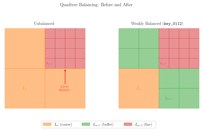
The figure shows the 2D quadtree analogue. Balancing inserts intermediate cells — the buffer level — wherever a coarse cell at would otherwise abut a fine cell at directly, so that no two neighbors differ by more than one level.
Strong balancing is the more restrictive condition, so it refines more cells and yields a larger mesh. In exchange, it admits a strictly smaller set of dual templates, and therefore guarantees better interior quality:
| Weak (default) | Strong (--strong) | |
|---|---|---|
| Neighbors constrained | face | face, edge, vertex |
| Distinct template configurations | 12 | 10 |
| Guaranteed interior minimum scaled Jacobian | ||
| Relative mesh size | smaller | larger |
For the Stanford bunny at --scale 10, strong balancing produced about 11% more elements at the dualization stage than weak — a modest cost for eliminating the two lowest-quality template configurations entirely. When interior element quality matters, prefer --strong. The catalogs behind this table are given in Template Quality.
Note that the two bounds coincide on simple convex geometry: a sphere attains under either rule. The distinction only emerges on topologically complex models — which are precisely the models where quality is hardest to recover afterward.
Pairing
Pairing ensures that transition regions are configured such that a dual template exists for every cell. automesh uses the regular pairing rule.
The two conditions interact: enforcing one can violate the other. Equilibration therefore alternates between balancing and pairing, repeating until a pass makes no further change — a fixed point — rather than applying each once in sequence.
Previous: Octree Construction. Next: Dualization, which converts the equilibrated octree into hexahedra.
Dualization
Stage 3 of five — the pivot. Consumes cells, emits hexahedra. See Hexahedral Meshing from a Surface for the pipeline overview and terminology.
With the octree equilibrated, the dual mesh is assembled as described in Two Meshes, Two Vocabularies: a node is placed at the center of every leaf cell, and hexahedra are formed around the octree's vertices.
Where eight equally sized leaf cells meet at a vertex, the hexahedron is immediate — join the eight cell centers, and the result is a cube. The difficulty is at transitions, where cells of differing refinement level meet and no such clean set of eight exists. Templates resolve these cases, and are applied in three passes:
- Face templates, for transitions across a shared face — two configurations, FT0 and FT1,
- Edge templates, for transitions along a shared edge — four configurations, ET1–ET4, and
- Vertex templates, for transitions at a shared vertex, including the star configuration.
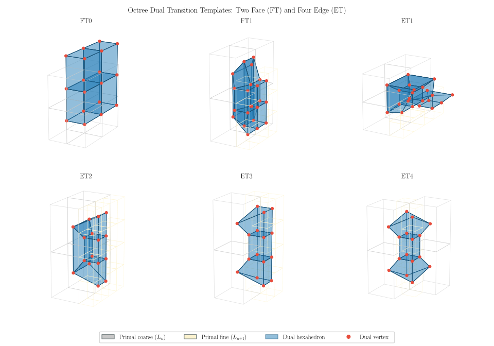
The figure shows the two face and four edge templates. In each panel the primal octree cells are drawn as wireframes — gray for the coarse level , pale yellow for the fine level — with the dual hexahedron shaded blue and its dual vertices marked in red. Reading a panel is a direct illustration of the dual correspondence: every red vertex sits at the center of a primal cell, and the blue element spans the primal vertex where those cells meet.
A fifth edge template exists under weak balancing. The four templates above are the complete set under
--strong. Weak balancing — the default — additionally admits a fifth edge configuration that strong balancing rules out. This is the structural reason the two balancing modes have different quality bounds: the extra template is the source of the sub- configurations reported in Template Quality.
This is why equilibration must precede dualization: balancing and pairing exist precisely to guarantee that every transition in the octree matches some template in the catalog. An unbalanced or unpaired octree can present configurations no template covers.
Every hexahedron in the interior of the mesh therefore comes from a finite catalog of local configurations, each with fixed geometry. This is the central property of the method: the interior mesh quality does not depend on the input surface at all. The catalog and the quality bound it guarantees are tabulated in Template Quality.
Once this stage completes, the octree has served its purpose and is not consulted again.
Previous: Equilibration. Next: Trimming, which discards the hexahedra lying outside the surface.
Trimming
Stage 4 of five. Operates on hexahedra. See Hexahedral Meshing from a Surface for the pipeline overview and terminology.
The octree is built over the bounding box of the surface, not the surface itself, so dualization produces hexahedra throughout that box — including regions outside the solid. Trimming discards them.
From this stage onward the octree is no longer consulted; trimming and buffering operate purely on the dual hexahedra.
Each dual node is classified inside or outside by casting rays against a bounding volume hierarchy of the surface and inspecting the orientation of the first facet hit. Three separate ray directions are used, and rays that graze a facet nearly tangentially are rejected in favor of the next direction — a single ray is not robust against grazing hits and coincident facets.
A hexahedron is then retained only if every one of its eight nodes is inside and every node clears the surface by at least half the length of the element's shortest edge. This clearance margin reserves room for the buffer layer that follows.
Trimming only removes elements; it never moves a node. Elements that survive trimming retain exactly their template geometry, and therefore their guaranteed quality.
Previous: Dualization. Next: Buffering, which fits the trimmed boundary to the surface.
Buffering
Stage 5 of five. Operates on hexahedra. See Hexahedral Meshing from a Surface for the pipeline overview and terminology.
Trimming leaves a blocky, stair-stepped boundary that does not follow the surface. Buffering resolves this by adding one conforming layer:
- The exterior faces of the trimmed mesh are extracted.
- Each boundary node is projected to its closest point on the surface.
- A hexahedron is extruded from each boundary face out to the projected nodes.
Before projecting, the extracted boundary is checked for manifoldness: every edge must be shared by exactly two faces. If not, meshing fails with
Error: non-manifold boundary.
This check is on the output boundary, not the input surface, and it is the only manifoldness test in the pipeline. It is a common failure — see Failure Modes.
The buffer elements are the only elements whose geometry is fitted to the surface, and consequently the only elements whose quality is unbounded. A poorly resolved or highly curved surface region will show up here and nowhere else.
Previous: Trimming. This is the final stage; the mesh is written out from here. For what to do with the result, see Quality Assessment and Improvement.
Dualization
Dualization is the process of using a primal mesh to construct a dual mesh. Dualization can be performed on 2D/3D surface meshes composed of quadrilateral elements, and 3D volumetric meshes composed of hexahedral elements. Both quadrilateral and hexahedral elements will be discussed.
Quadtree
With plot_quadtree_convention.py, we create the following index scheme:
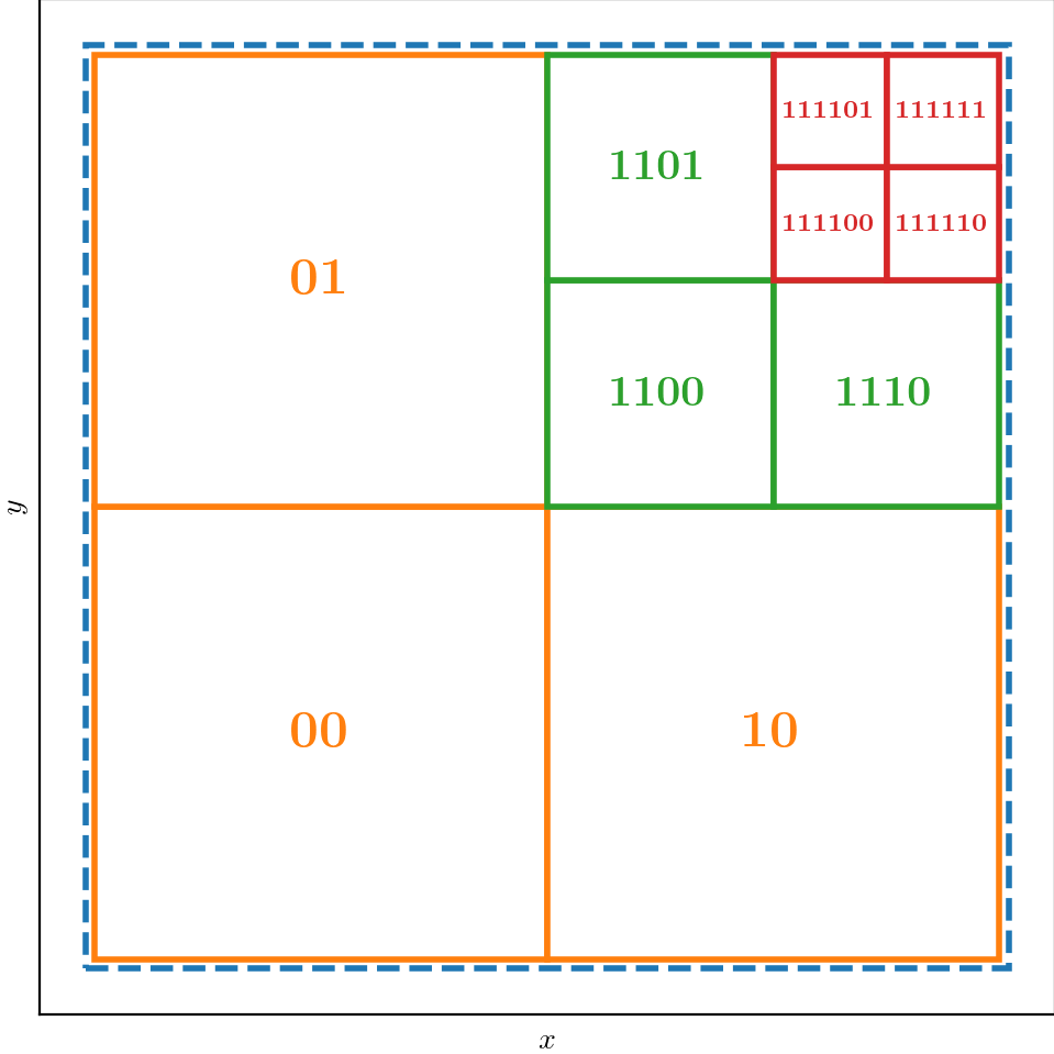
With fig_quadtree.tex, we create the following image of the inverted tree:
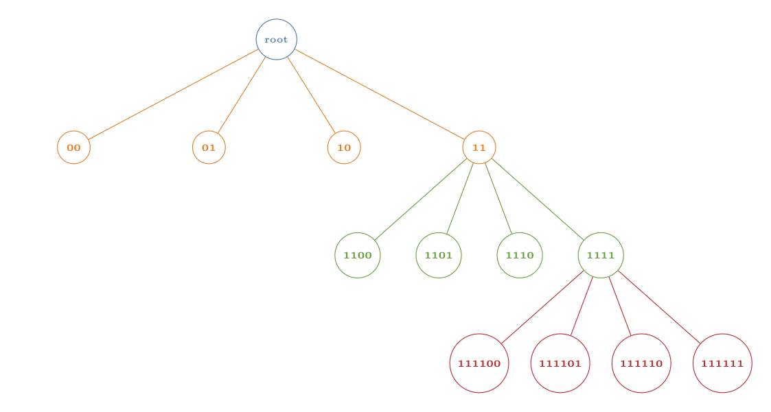
With plot_quadtree.py, we plot a domain
- A square domain
L0 - Single point at
(2.6, 0.6)to trigger refinement.
| Level 0 | 1 | 2 |
|---|---|---|
 |  |  |
| 3 | 4 | 5 |
|---|---|---|
 |  |  |
Circle from Segmentation
We illustrate the segmentation start point as it applies to quadtree formation.
- For a segmentation at a given resolution of pixels, we immerse the segmentation into a single-cell (
L0) quadtree domain. - We pad the segmentation margins with void (segmentation ID
0) such that the pixel count in all directions ( and )- is the same, and
- is divisible by 2 for cell subdivisions.
- For each cell in the quadtree, we process the cells recursively and ask this question: Does the cell contain more than one material? If yes, then subdivide; if no, then do not subdivide.
| 3 | 4 | 5 | 6 |
|---|---|---|---|
 | 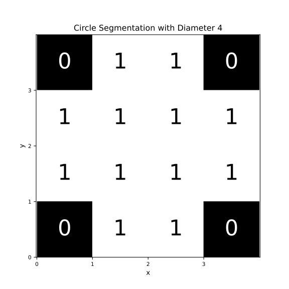 | 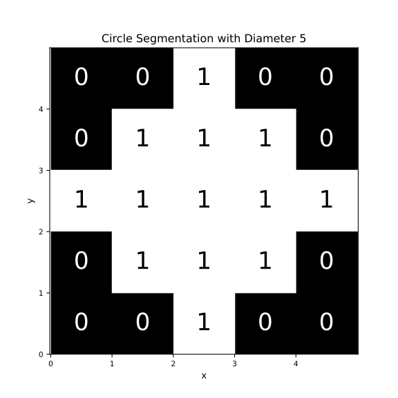 | 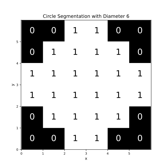 |
| 13 | 14 | 15 | 16 |
|---|---|---|---|
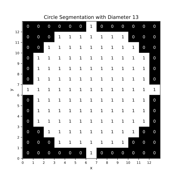 | 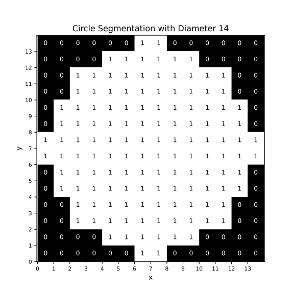 | 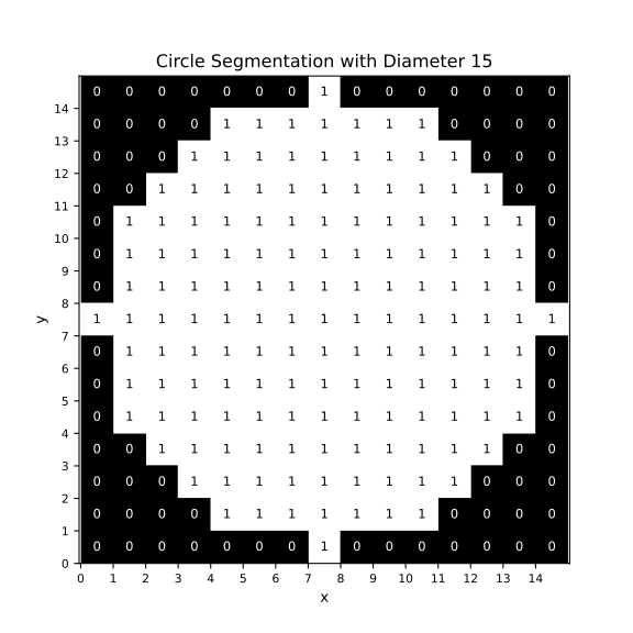 | 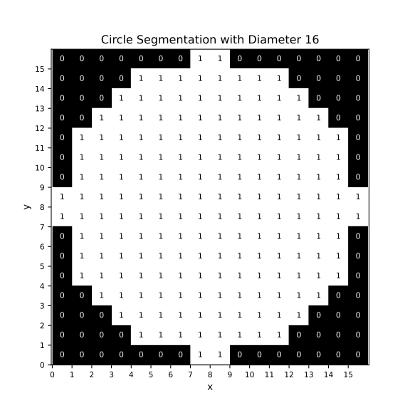 |
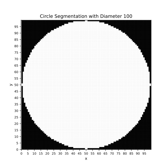
Circle from Boundary
We illustrate the boundary start point as it applies to quadtree formation.
- We define a boundary as directed series of connected, discrete points that create a closed-loop, non-intersecting path.
- We immerse the boundary into a single-cell (
L0) quadtree domain. - For each cell in the quadtree, we process the cells recursively and ask this question: Does the cell contain at least one boundary point? If yes, then subdivide; if no, then do not subdivide.
Consider a boundary of a circle defined by discrete (x, y) points.
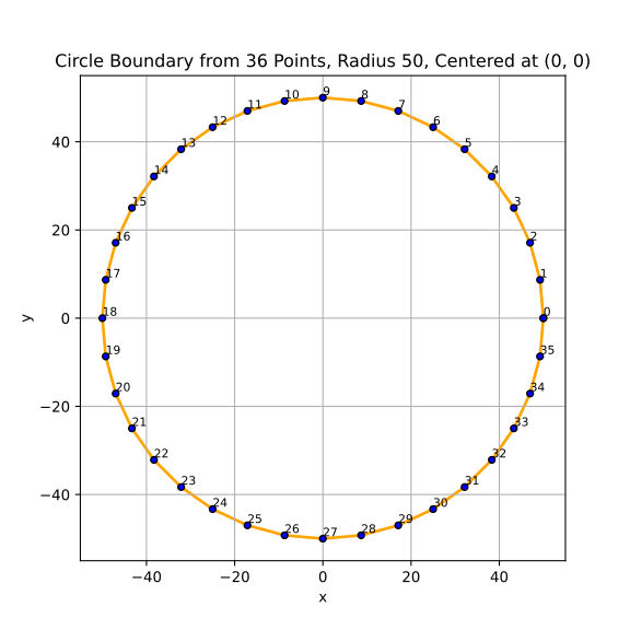
| Level 0 | 1 | 2 |
|---|---|---|
 |  |  |
| 3 | 4 | 5 |
|---|---|---|
 | 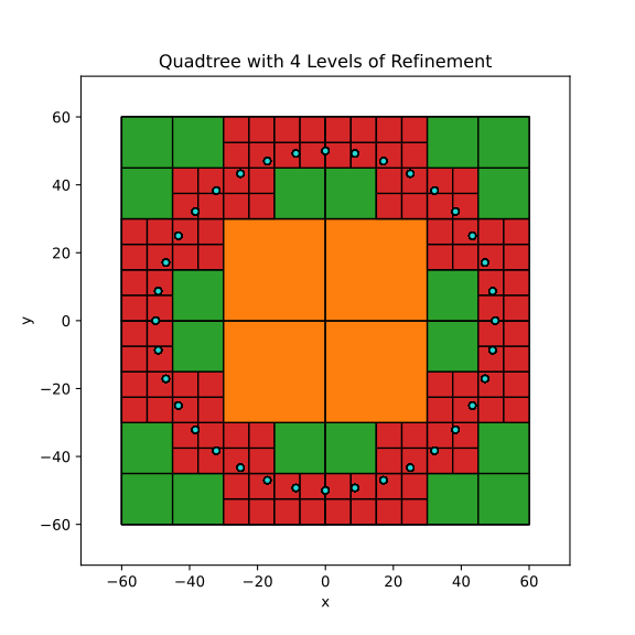 | 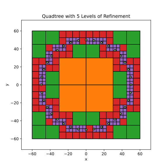 |
Circle from Tessellation
We illustrate the tessellation as it applies to quadtree formation.
- We immerse the tessellation into a single-cell (
L0) quadtree domain. - We create a boundary of the tessellation with points that lie on the boundary of the tessellation.
- We immerse the boundary into a single-cell (
L0) quadtree domain. - For each cell in the quadtree, we process the cells recursively and ask this question: Does the cell contain at least one boundary point? If yes, then subdivide; if no, then do not subdivide.
Quarter Plate
With Python, we produce a Quadtree with zero to five levels of refinement. Refinement is triggered based on whether or not a cell contains one or more seed points, shown as points along the quarter circle centered at (4, 0).
| Level 0 | 1 | 2 |
|---|---|---|
 |  | 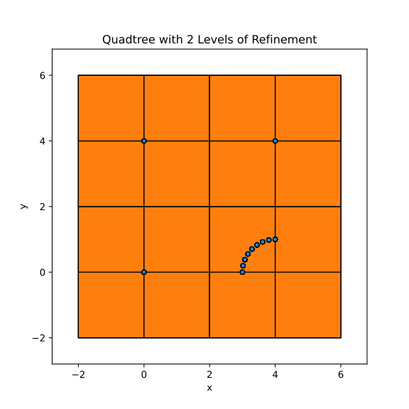 |
| 3 | 4 | 5 |
|---|---|---|
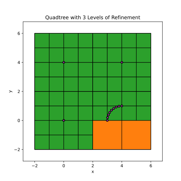 | 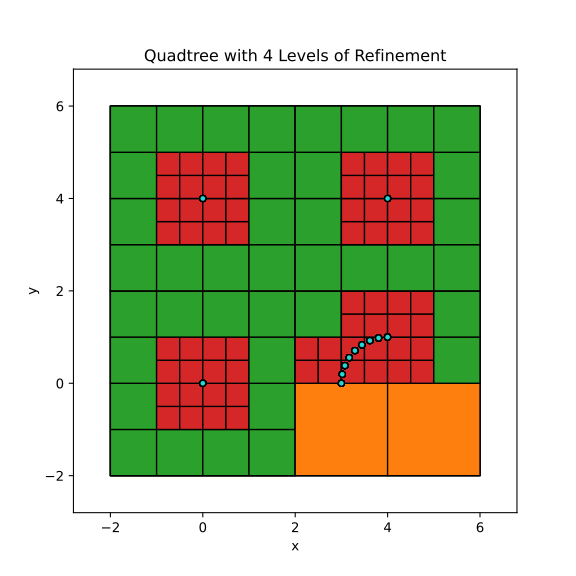 | 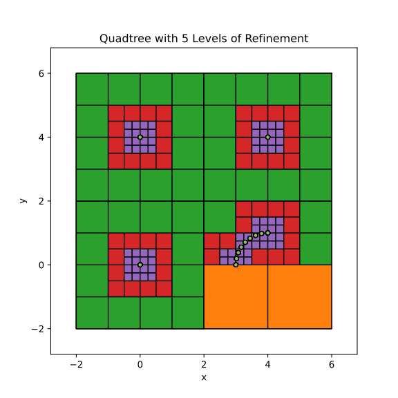 |
Octree
Sphere
Consider a boundary of a sphere defined by a discrete triangular tessellation.
References
- https://github.com/sandialabs/sibl/blob/master/geo/doc/quadtree.md
- https://github.com/sandialabs/sibl/blob/master/geo/doc/dual_quad_transitions.md
- https://github.com/sandialabs/sibl/blob/master/geo/doc/dual/lesson_11.md
Source
quadtree_plot.py
quadtree_plot.py
"""This module creates a quadtree and plots it."""

from pathlib import Path
from typing import NamedTuple


import matplotlib.pyplot as plt
from matplotlib import patches
import numpy as np

# from book.dualization.code.color_schemes import QuadColors
from color_complement import ColorComplement
from color_schemes import ColorSchemes, DiscreteColors


class Point(NamedTuple):
    """A point in 2D space."""

    x: float  # x-coordinate
    y: float  # y-coordinate


class Boundary(NamedTuple):
    """A boundary defined by its minimum and maximum
    x and y coordinates."""

    xmin: float  # Minimum x-coordinate
    xmax: float  # Maximum x-coordinate

    ymin: float  # Minimum y-coordinate
    ymax: float  # Maximum y-coordinate


class QuadTree:
    """Defines a quadtree composed of a single parent quad and recursive
    children quads.
    """

    def __init__(
        self,
        *,
        x: float,
        y: float,
        width: float,
        height: float,
        level: int,
        max_level: int,
        seeds: list[Point],
        verbose: bool,
    ):
        # (x, y, width, height)
        self.boundary = Boundary(xmin=x, xmax=x + width, ymin=y, ymax=y + height)
        self.level = level
        self.max_level = max_level
        self.has_children = False
        self.children = []
        assert level <= max_level, (
            f"QuadTree level {level} exceeds max_level {max_level}."
        )
        self.verbose = verbose

        if self.contains_any_point(seeds):
            # If the quad contains any of the seed points, subdivide it
            self.subdivide(seeds=seeds)

    def subdivide(self, seeds: list[Point]):
        """Divides the parent quad into four quad children."""
        if self.level < self.max_level:
            if self.verbose:
                print(
                    f"Subdividing quad at level {self.level} with boundary {self.boundary}"
                )
            x = self.boundary.xmin
            y = self.boundary.ymin
            width = self.boundary.xmax - self.boundary.xmin
            height = self.boundary.ymax - self.boundary.ymin
            half_width = width / 2.0
            half_height = height / 2.0

            self.has_children = True  # overwrite

            # Create four children
            self.children.append(
                QuadTree(
                    x=x,
                    y=y,
                    width=half_width,
                    height=half_height,
                    level=self.level + 1,
                    max_level=self.max_level,
                    seeds=seeds,
                    verbose=self.verbose,
                )
            )  # Top-left
            self.children.append(
                QuadTree(
                    x=x + half_width,
                    y=y,
                    width=half_width,
                    height=half_height,
                    level=self.level + 1,
                    max_level=self.max_level,
                    seeds=seeds,
                    verbose=self.verbose,
                )
            )  # Top-right
            self.children.append(
                QuadTree(
                    x=x,
                    y=y + half_height,
                    width=half_width,
                    height=half_height,
                    level=self.level + 1,
                    max_level=self.max_level,
                    seeds=seeds,
                    verbose=self.verbose,
                )
            )  # Bottom-left
            self.children.append(
                QuadTree(
                    x=x + half_width,
                    y=y + half_height,
                    width=half_width,
                    height=half_height,
                    level=self.level + 1,
                    max_level=self.max_level,
                    seeds=seeds,
                    verbose=self.verbose,
                )
            )  # Bottom-right

    def contains(self, point: Point) -> bool:
        """Check if the quadtree contains a point."""
        # TODO: determine if we want this to be consistent with
        # winding number conventions
        return (
            point.x >= self.boundary.xmin
            and point.x <= self.boundary.xmax
            and point.y >= self.boundary.ymin
            and point.y <= self.boundary.ymax
        )

    def contains_any_point(self, points: list[Point]) -> bool:
        """Check if the quadtree contains any of the given points.
        Python's built-in any() short-circuits: it returns True as
        soon as it finds the first truthy value and stops evaluating the rest.

        """
        # result = any(self.contains(point) for point in points)
        # return result
        return any(self.contains(point) for point in points)

    def draw(self, ax, quadcolors: DiscreteColors, seeds: list[Point] | None):
        """Draw the quadtree."""
        x = self.boundary.xmin
        y = self.boundary.ymin
        width = self.boundary.xmax - self.boundary.xmin
        height = self.boundary.ymax - self.boundary.ymin
        # Draw the boundary rectangle
        if self.verbose:
            print(
                f"Drawing level {self.level} quad at ({x}, {y}) with width {width} and height {height}"
            )
        rect = patches.Rectangle(
            (x, y),
            width,
            height,
            # linewidth=1,
            linestyle="solid",
            edgecolor=quadcolors.edgecolor,
            # facecolor=ColorComplement.hex_complement(
            #     quadcolors.facecolors[self.level], "hsv"
            # ),
            facecolor=quadcolors.facecolors[self.level],
            alpha=quadcolors.alpha,
            zorder=2,
        )
        ax.add_patch(rect)

        # Draw children
        if self.has_children:
            if self.verbose:
                print(f"Quad at level {self.level} has children, drawing them.")
            for child in self.children:
                child.draw(ax, quadcolors, seeds)

        # Draw the seed points, only draw them after we have reached
        # the top level of the quadtree to avoid cluttering the plot
        # with too many points at lower levels.
        if seeds is not None and self.level == self.max_level:
            xs = [seed.x for seed in seeds]
            ys = [seed.y for seed in seeds]
            ax.scatter(
                xs,
                ys,
                marker="o",
                edgecolor=quadcolors.edgecolor,
                color=ColorComplement.hex_complement(
                    quadcolors.facecolors[self.level], "hsv"
                ),
                alpha=quadcolors.alpha,
                s=20,  # Adjust size as needed
                zorder=3,
            )


class Configuration(NamedTuple):
    """User input configuration for the quadtree plot."""

    xmin: float  # Minimum x-coordinate for the quadtree
    xmax: float  # Maximum x-coordinate for the quadtree
    ymin: float  # Minimum y-coordinate for the quadtree
    ymax: float  # Maximum y-coordinate for the quadtree

    level_min: int  # Minimum level of the quadtree
    level_max: int  # Maximum level of the quadtree

    seeds: list[Point]  # List of seed points for the quadtree

    fig_stem: str  # Stem for the filename when saving

    alpha: float = 1.0  # Transparency of the quadtree colors
    save: bool = True  # Whether to save the plot
    show: bool = True  # Whether to show the plot
    dpi: int = 300  # Dots per inch for saving the plot
    fig_width: float = 6.0  # Width of the figure in inches
    fig_height: float = 6.0  # Height of the figure in inches
    ext: str = ".svg"  # File extension for saving the plot

    verbose: bool = False  # Whether to print debug information


def quarter_plate_seeds() -> list[Point]:
    """Helper function to create seeds for the Hughes quarter plate example."""

    # Similar to the round in the Hughes quarter plate problem
    # https://github.com/sandialabs/sibl/blob/master/geo/doc/dual/lesson_11.md
    # see also Cottrell 2009 IGA book, page 117.
    radius = 1.0
    theta_start = np.pi / 2.0
    theta_stop = np.pi
    n_points = 9
    theta_values = np.linspace(theta_start, theta_stop, n_points)
    offset_x, offset_y = 4.0, 0.0
    seeds = [
        Point(x=radius * np.cos(theta) + offset_x, y=radius * np.sin(theta) + offset_y)
        for theta in theta_values
    ]
    corner_seeds = [
        Point(x=4, y=4),
        Point(x=0, y=4),
        Point(x=0, y=0),
    ]
    seeds += corner_seeds
    return seeds


def circle_seeds() -> list[Point]:
    """Helper function to create seeds for a circle."""

    # Create an array of angles from 0 to 2 pi
    center = (0, 0)
    radius = 50
    n_pts = 36
    theta = np.linspace(0, 2 * np.pi, n_pts + 1)

    # Parametric equations for the circle
    x = center[0] + radius * np.cos(theta)
    y = center[1] + radius * np.sin(theta)
    seeds = [Point(x=xi, y=yi) for xi, yi in zip(x, y)]
    return seeds


def main():
    # Circle example
    cc = Configuration(
        xmin=-60,
        xmax=60,
        ymin=-60,
        ymax=60,
        #
        level_min=0,
        level_max=5,
        #
        seeds=circle_seeds(),
        #
        fig_stem="quadtree_circle",
    )

    # Hughes quarter plate example
    _cc = Configuration(
        xmin=-2,
        xmax=6,
        ymin=-2,
        ymax=6,
        #
        level_min=0,
        level_max=4,
        #
        seeds=quarter_plate_seeds(),
        #
        fig_stem="quadtree_quarter_plate",
    )

    # Create a figure and axis
    fig, ax = plt.subplots(figsize=(cc.fig_width, cc.fig_height))

    # Create the quadtree with a boundary of (-12, -12, 24, 24)
    qt = QuadTree(
        x=cc.xmin,
        y=cc.ymin,
        width=cc.xmax - cc.xmin,
        height=cc.ymax - cc.ymin,
        level=cc.level_min,
        max_level=cc.level_max,
        verbose=cc.verbose,
        seeds=cc.seeds,
    )

    # The number of colors will be the number of levels + 1 because
    # the root level is 0 and we want to include it in the color palette
    # n_colors = level_max - level_min + 2
    n_colors = 10  # Number of discrete colors to extract
    qc = DiscreteColors(
        n_levels=n_colors,
        edgecolor="black",
        alpha=cc.alpha,
        color_scheme=ColorSchemes.TAB10,
        reversed=False,
    )
    if cc.verbose:
        print(f"quadcolors.facecolors: {qc.facecolors}")
    # Draw the quadtree
    qt.draw(ax=ax, quadcolors=qc, seeds=cc.seeds)

    # Set limits and aspect
    margin = 0.1 * (cc.xmax - cc.xmin)
    ax.set_xlim(cc.xmin - margin, cc.xmax + margin)
    ax.set_ylim(cc.ymin - margin, cc.ymax + margin)
    ax.set_aspect("equal")
    ax.set_xlabel("x")
    ax.set_ylabel("y")
    # Turn grid to off
    ax.grid(False)
    # ax.set_xticks([])
    # ax.set_yticks([])
    GRAMMAR_LEVELS = (
        f"{cc.level_max} Level" if cc.level_max == 1 else f"{cc.level_max} Levels"
    )
    ax.set_title(f"Quadtree with {GRAMMAR_LEVELS} of Refinement")
    plt.show()

    if cc.show:
        plt.show()

    if cc.save:
        parent = Path(__file__).parent
        # stem = Path(__file__).stem + "_level_" + str(cc.level_max)
        stem = cc.fig_stem + "_level_" + str(cc.level_max)
        fn = parent.joinpath(stem + cc.ext)
        # plt.savefig(fn, dpi=DPI, bbox_inches='tight')
        fig.savefig(fn, dpi=cc.dpi)
        print(f"Saved {fn}")


if __name__ == "__main__":
    main()
Smoothing
Both Laplacian smoothing1 and Taubin smoothing2 3 are smoothing operations that adjust the positions of the nodes in a finite element mesh.
Laplacian smoothing, based on the Laplacian operator, computes the average position of a point's neighbors and moves the point toward the average. This reduces high-frequency noise but can result in a loss of shape and detail, with overall shrinkage.
Taubin smoothing is an extension of Laplacian smoothing that seeks to overcome the shrinkage drawback associated with the Laplacian approach. Taubin is a two-pass approach. The first pass smooths the mesh. The second pass re-expands the mesh.
Laplacian Smoothing
Consider a subject node with position . The subject node connects to neighbor points for through edges.
For concreteness, consider a node with four neighbors, shown in the figure below.
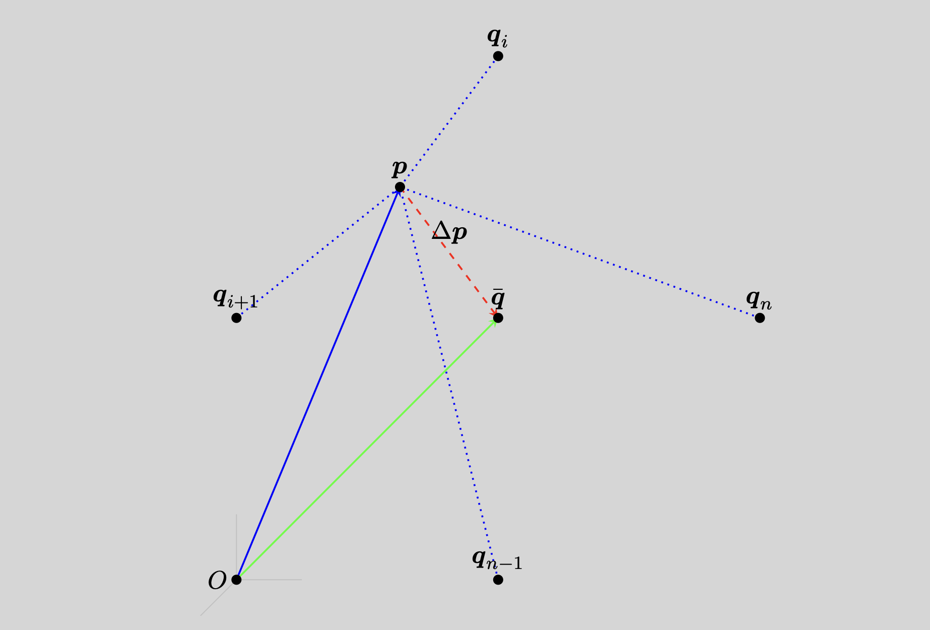
Figure 11-1: The subject node with edge connections (dotted lines) to neighbor nodes with (without loss of generality, the specific example of is shown). The average position of all neighbors of is denoted , and the gap (dashed line) originates at and terminates at .
Define as the average position of all neighbors of ,
Define the gap vector as originating at and terminating at (viz., ),
Let be the positive scaling factor for the gap .
Since
subdivision of this relationship into several substeps gives rise to an iterative approach. We typically select to avoid overshoot of the update, .
At iteration , we update the position of by an amount to as
with
Thus
and finally
The formulation above, based on the average position of the neighbors, is a special case of the more generalized presentation of Laplace smoothing, wherein a normalized weighting factor, , is used:
When all weights are equal and normalized by the number of neighbors, , the special case presented in the box above is recovered.
Example
For a 1D configuration, consider a node with initial position with two neighbors (that never move) with positions and (). With , the table below shows updates for for position .
Table: Iteration updates of a 1D example.
| 0 | 0.5 | 1.5 | -1 | -0.3 |
| 1 | 0.5 | 1.2 | -0.7 | -0.21 |
| 2 | 0.5 | 0.99 | -0.49 | -0.147 |
| 3 | 0.5 | 0.843 | -0.343 | -0.1029 |
| 4 | 0.5 | 0.7401 | -0.2401 | -0.07203 |
| 5 | 0.5 | 0.66807 | -0.16807 | -0.050421 |
| 6 | 0.5 | 0.617649 | -0.117649 | -0.0352947 |
| 7 | 0.5 | 0.5823543 | -0.0823543 | -0.02470629 |
| 8 | 0.5 | 0.55764801 | -0.05764801 | -0.017294403 |
| 9 | 0.5 | 0.540353607 | -0.040353607 | -0.012106082 |
| 10 | 0.5 | 0.528247525 | -0.028247525 | -0.008474257 |
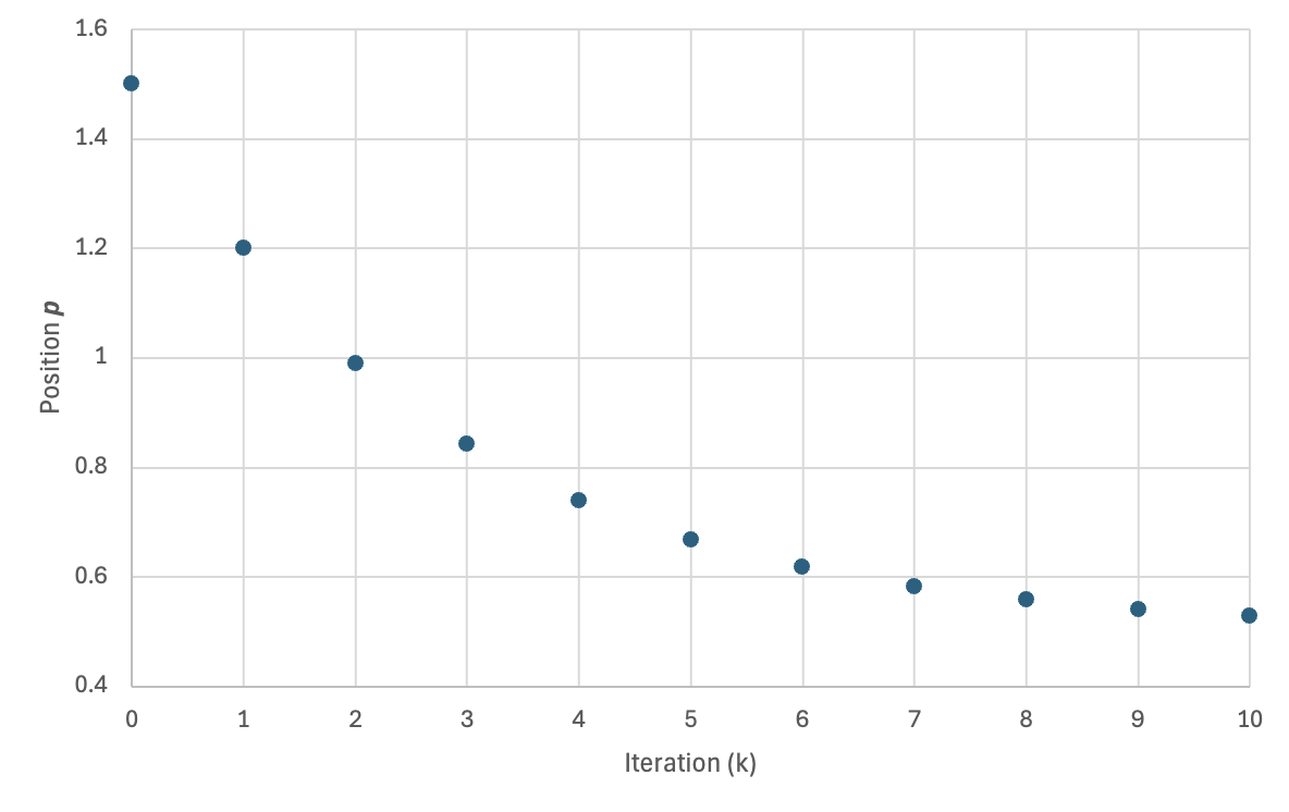
Figure 11-2: Convergence of position toward as a function of iteration .
Taubin Smoothing
Taubin smoothing is a two-parameter, two-pass iterative variation of Laplace smoothing. Specifically with the definitions used in Laplacian smoothing, a second negative parameter is used, where
The first parameter, , tends to smooth (and shrink) the domain. The second parameter, , tends to expand the domain.
Taubin smoothing is written, for , , , with typically being even, as
- First pass (if is even):
- Second pass (if is odd):
In any second pass (any pass with odd), the algorithm uses the updated positions from the previous (even) iteration to compute the new positions. So, the average is taken from the updated neighbor positions rather than the original neighbor positions. Some presentation of Taubin smoothing do not carefully state the second pass update, and so we emphasize it here.
Taubin Parameters
We follow the recommendations of Taubin3 for selecting values of and , with specific details noted as follows: We use the second degree polynomial transfer function,
with as the domain of interest since the eigenvalues of the discrete Laplacian being approximated all are within .3
There is a value of called the pass-band frequency, ,
such that for all values of and .
Given that , the pass-band and
Taubin noted that values of "...from 0.01 to 0.1 produce good results, and all examples shown in this paper were computed with ." Taubin also noted that for , choice of such that "...ensures a stable and fast filter."
We implement the following default values:
- ,
which provides and .
Hierarchical Control
As a default, all nodes in the mesh are free nodes, meaning they are subject to updates in position due to smoothing.
- Free nodes
For the purpose of hierarchical smoothing, we categorize all nodes as belonging to one of the following categories.
- Boundary nodes
- Nodes on the exterior of the domain and nodes that lie at the interface of two different blocks are reclassified from free nodes to boundary nodes.
- Like free nodes, these nodes are also subject to updates in position due to smoothing.
- Unlike free nodes, which are influenced by positions of neighboring nodes of any category, boundary nodes are only influenced positions of other boundary nodes, or prescribed nodes (described below).
- Interior nodes
- The free nodes not categorized as boundary nodes are categorized as interior nodes.
- Interior nodes are influenced by neighboring nodes of all categories.
- Prescribed nodes
- Finally, we may wish to select nodes, typically but not necessarily from boundary nodes, to move to a specific location, often to match the desired shape of a mesh. These nodes are reclassified as prescribed nodes.
- Prescribed nodes are not subject to updates in position due to smoothing because they are a priori prescribed to reside at a given location.
This classification is shown below in figures. All nodes in the mesh are categorized as FREE nodes:
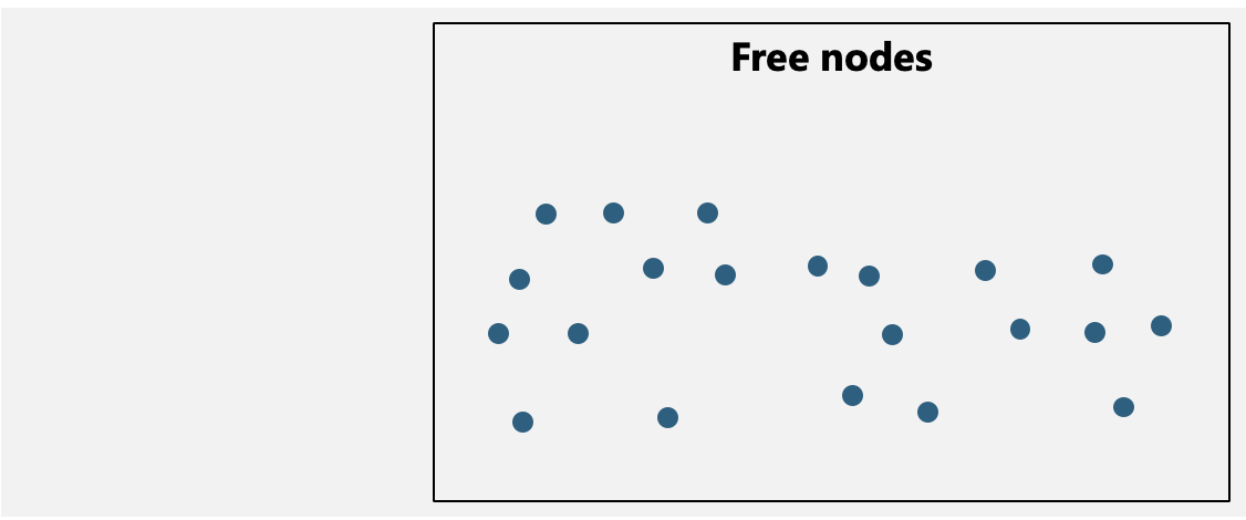
Nodes that lie on the exterior and/or an interface are categorized as BOUNDARY nodes. The remaining free nodes that are not BOUNDARY nodes are INTERIOR nodes.
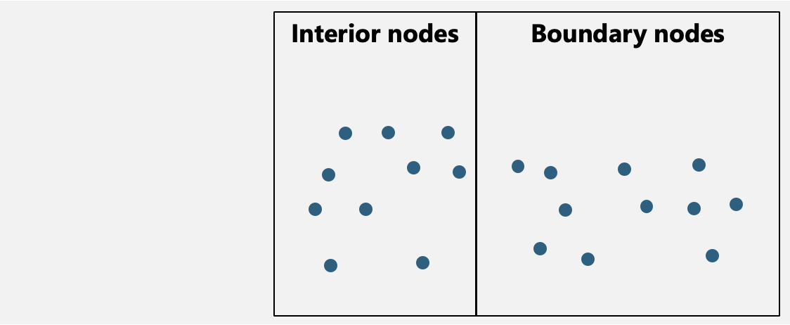
Some INTERIOR and BOUNDARY nodes may be recategorized as PRESCRIBED nodes.
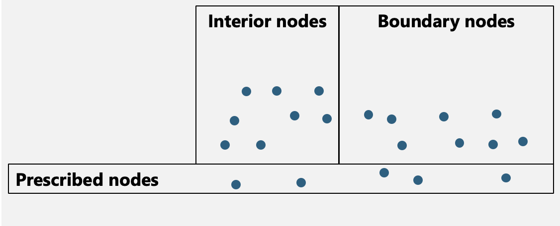
Note that this focuses on regular volumetric finite element meshes, and does not apply to certain other meshes. For example, manifold surface meshes embedded in three dimensions have only interior nodes, so hierarchical control would not apply.
The Hierarchy enum
These three categories, INTERIOR, BOUNDARY, and PRESCRIBED, compose the hierarchical structure of hierarchical smoothing. Nodes are classified in code with the following enum,
class Hierarchy(Enum):
    """All nodes must be categorized as belonging to one, and only one,
    of the following hierarchical categories.
    """

    INTERIOR = 0
    BOUNDARY = 1
    PRESCRIBED = 2
Hierarchical Control
Hierarchical control classifies all nodes in a mesh as belonging to a interior , boundary , or prescribed . These categories are mutually exclusive. Any and all nodes must belong to one, and only one, of these three categories. For a given node , let
- the set of interior neighbors be denoted ,
- the set of boundary neighbors be denoted , and
- the set of prescribed neighbors be denoted .
Hierarchical control redefines a node's neighborhood according to the following hierarchical rules:
- for any interior node , nodes , , and are neighbors; there is no change in the neighborhood,
- for any boundary node , only boundary nodes and prescribed nodes are neighbors; a boundary node neighborhood excludes interior nodes, and
- for any prescribed node , all neighbors of any category are excluded; the prescribed node's position does not change during smoothing.
The following figure shows this concept:
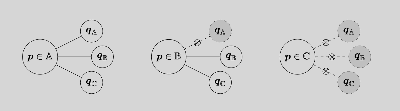
Figure 11-3: Classification of nodes into categories of interior nodes , boundary nodes , and prescribed nodes . Hierarchical relationship: An interior node's smoothing neighbors are nodes of any category, a boundary node's smoothing neighbors are other boundary nodes or other prescribed nodes, and prescribed nodes have no smoothing neighbors.
Relationship to a SideSet
A SideSet is a set of nodes on the boundary of a domain, used to prescribe a boundary condition on the finite element mesh.
- A subset of nodes on the boundary nodes is classified as exterior nodes.
- A different subset of nodes on the boundary is classified as interface nodes.
- A
SideSetis composed of either exterior nodes or interface nodes. - Because a node can lie both on the exterior and on an interface, some nodes (shown in red) are included in both the exterior nodes and the interface nodes.

Chen Example
Chen4 used medical image voxel data to create a structured hexahedral mesh. They noted that the approach generated a mesh with "jagged edges on mesh surface and material interfaces," which can cause numerical artifacts.
Chen used hierarchical Taubin mesh smoothing for eight (8) iterations, with and to smooth the outer and inner surfaces of the mesh.
References
-
Sorkine O. Laplacian mesh processing. Eurographics (State of the Art Reports). 2005 Sep;4(4):1. paper ↩
-
Taubin G. Curve and surface smoothing without shrinkage. In Proceedings of IEEE international conference on computer vision 1995 Jun 20 (pp. 852-857). IEEE. paper ↩
-
Taubin G. A signal processing approach to fair surface design. In Proceedings of the 22nd annual conference on Computer graphics and interactive techniques 1995 Sep 15 (pp. 351-358). paper ↩ ↩2 ↩3
-
Chen Y, Ostoja-Starzewski M. MRI-based finite element modeling of head trauma: spherically focusing shear waves. Acta mechanica. 2010 Aug;213(1):155-67. paper ↩
Hexahedral Metrics
automesh metrics hex --help
automesh implements the following hexahedral element quality metrics1:
- Maximum edge ratio
- Minimum scaled Jacobian
- Maximum skew
- Element volume
A brief description of each metric follows.
Maximum Edge Ratio
- measures the ratio of the longest edge to the shortest edge in a mesh element.
- A ratio of 1.0 indicates perfect element quality, whereas a very large ratio indicates bad element quality.
- Knupp et al.1 (page 87) indicate an acceptable range of
[1.0, 1.3].
Minimum Scaled Jacobian
- evaluates the determinant of the Jacobian matrix at each of the corners nodes, normalized by the corresponding edge lengths, and returns the minimum value of those evaluations.
- Interpretation
- : Perfect rectangular element
- : Element is valid (positive Jacobian)
- : Element zero volume
- : Invalid element (inverted/negative Jacobian)
Typically, mesh quality requirements specify for acceptable elements.
- Knupp et al.1 (page 92) indicate an acceptable range of
[0.5, 1.0], though in practice, minimum values as low as0.2and0.3are often used.
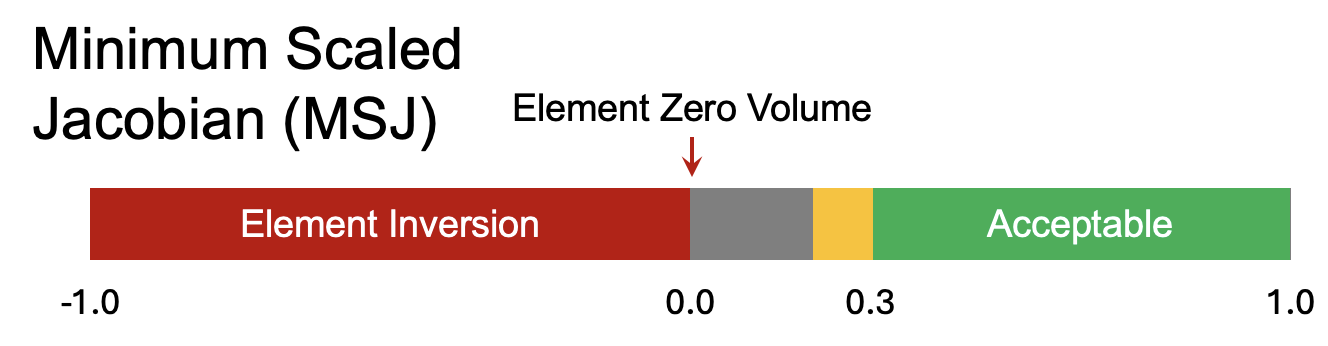
Figure 12-1: Illustration of minimum scaled Jacobian2 with acceptable range [0.3, 1.0].
Maximum Skew
- Skew measures how much an element deviates from being a regular shape (e.g., in 3D, a cube or regular tetrahedron; in 2D, a square or equilateral triangle). A skew value of 0 indicates a perfectly regular shape, while higher values indicate increasing levels of distortion.
- Knupp et al.1 (page 97) indicate an acceptable range of
[0.0, 0.5].
Element Volume
- Measures the volume of the element.
Unit Tests
Inspired by Figure 2 of Livesu et al.3 reproduced here below
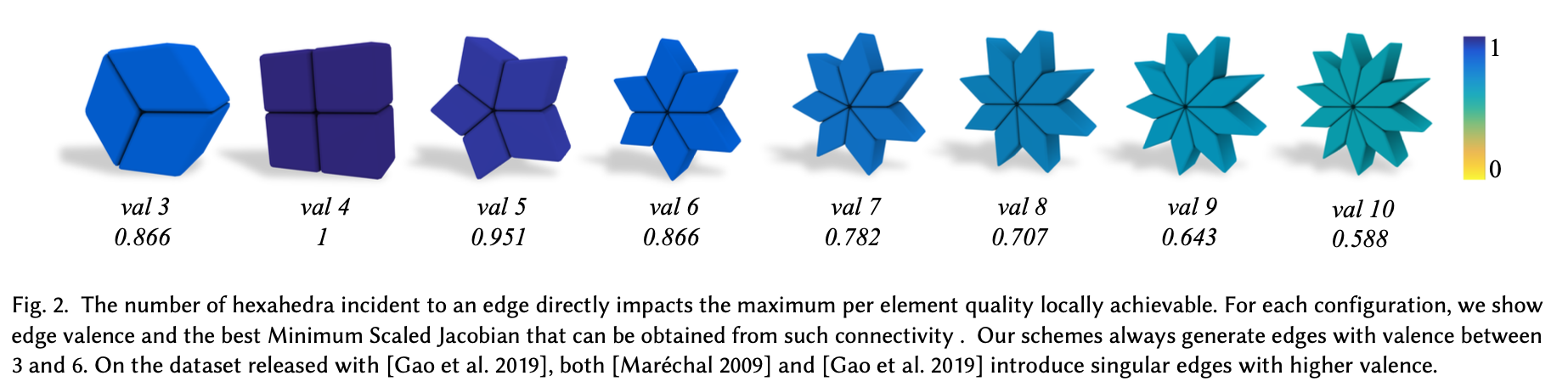
we examine several unit test singleton elements and their metrics.
| valence | singleton | volume | |||
|---|---|---|---|---|---|
| 3 |  | 1.000000e0 (1.000) | 8.660253e-1 (0.866) | 5.000002e-1 (0.500) | 8.660250e-1 (0.866) |
| 3' (noised) |  | 1.292260e0 (2.325) ** Cubit (aspect ratio): 1.292 | 1.917367e-1 (0.192) | 6.797483e-1 (0.680) | 1.247800e0 (1.248) |
| 4 |  | 1.000000e0 (1.000) | 1.000000e0 (1.000) | 0.000000e0 (0.000) | 1.000000e0 (1.000) |
| 4' (noised) |  | 1.167884e0 (1.727) ** Cubit (aspect ratio): 1.168 | 3.743932e-1 (0.374) | 4.864936e-1 (0.486) | 9.844008e-1 (0.984) |
| 5 | 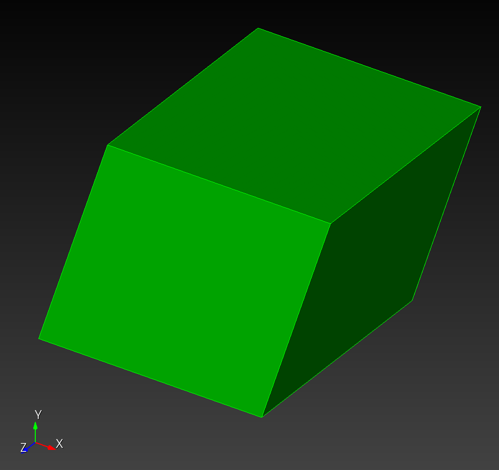 | 1.000000e0 (1.000) | 9.510566e-1 (0.951) | 3.090169e-1 (0.309) | 9.510570e-1 (0.951) |
| 6 | 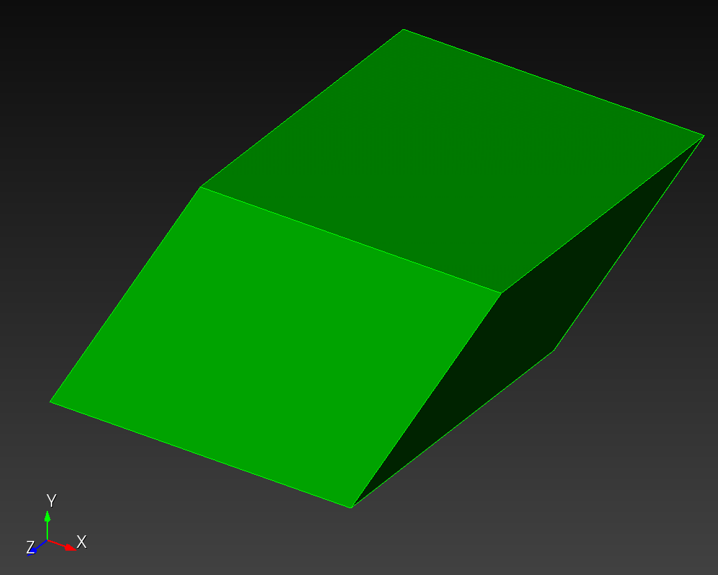 | 1.000000e0 (1.000) | 8.660253e-1 (0.866) | 5.000002e-1 (0.500) | 8.660250e-1 (0.866) |
| ... | ... | ... | ... | ... | ... |
| 10 | 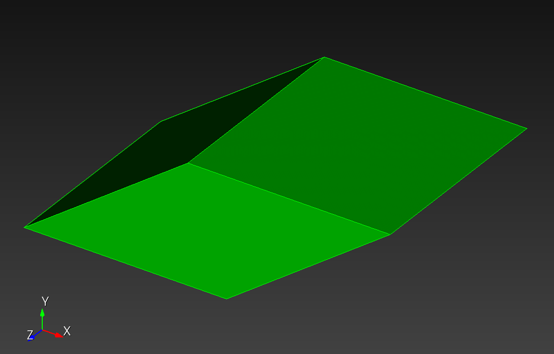 | 1.000000e0 (1.000) | 5.877851e-1 (0.588) | 8.090171e-1 (0.809) | 5.877850e-1 (0.588) |
Figure 12-2: Hexahedral metrics. Leading values are from automesh. Values in parenthesis are results from HexaLab.4 Items with ** indicate where automesh and Cubit agree, but HexaLab disagrees. Cubit uses the term Aspect Ratio for Edge Ratio for hexahedral elements. All values were also verified with Cubit.
The connectivity for all elements:
1, 2, 4, 3, 5, 6, 8, 7
with prototype:

The element coordinates follow:
# 3
    1,      0.000000e0,      0.000000e0,      0.000000e0
    2,      1.000000e0,      0.000000e0,      0.000000e0
    3,     -0.500000e0,      0.866025e0,      0.000000e0
    4,      0.500000e0,      0.866025e0,      0.000000e0
    5,      0.000000e0,      0.000000e0,      1.000000e0
    6,      1.000000e0,      0.000000e0,      1.000000e0
    7,     -0.500000e0,      0.866025e0,      1.000000e0
    8,      0.500000e0,      0.866025e0,      1.000000e0

# 3'
    1,      0.110000e0,      0.120000e0,     -0.130000e0
    2,      1.200000e0,     -0.200000e0,      0.000000e0
    3,     -0.500000e0,      1.866025e0,     -0.200000e0
    4,      0.500000e0,      0.866025e0,     -0.400000e0
    5,      0.000000e0,      0.000000e0,      1.000000e0
    6,      1.000000e0,      0.000000e0,      1.000000e0
    7,     -0.500000e0,      0.600000e0,      1.400000e0
    8,      0.500000e0,      0.866025e0,      1.200000e0

# 4
    1,      0.000000e0,      0.000000e0,      0.000000e0
    2,      1.000000e0,      0.000000e0,      0.000000e0
    3,      0.000000e0,      1.000000e0,      0.000000e0
    4,      1.000000e0,      1.000000e0,      0.000000e0
    5,      0.000000e0,      0.000000e0,      1.000000e0
    6,      1.000000e0,      0.000000e0,      1.000000e0
    7,      0.000000e0,      1.000000e0,      1.000000e0
    8,      1.000000e0,      1.000000e0,      1.000000e0

# 4'
    1,      0.100000e0,      0.200000e0,      0.300000e0
    2,      1.200000e0,      0.300000e0,      0.400000e0
    3,     -0.200000e0,      1.200000e0,     -0.100000e0
    4,      1.030000e0,      1.102000e0,     -0.250000e0
    5,     -0.001000e0,     -0.021000e0,      1.002000e0
    6,      1.200000e0,     -0.100000e0,      1.100000e0
    7,      0.000000e0,      1.000000e0,      1.000000e0
    8,      1.010000e0,      1.020000e0,      1.030000e0

# 5
    1,      0.000000e0,      0.000000e0,      0.000000e0
    2,      1.000000e0,      0.000000e0,      0.000000e0
    3,      0.309017e0,      0.951057e0,      0.000000e0
    4,      1.309017e0,      0.951057e0,      0.000000e0
    5,      0.000000e0,      0.000000e0,      1.000000e0
    6,      1.000000e0,      0.000000e0,      1.000000e0
    7,      0.309017e0,      0.951057e0,      1.000000e0
    8,      1.309017e0,      0.951057e0,      1.000000e0

# 6
    1,      0.000000e0,      0.000000e0,      0.000000e0
    2,      1.000000e0,      0.000000e0,      0.000000e0
    3,      0.500000e0,      0.866025e0,      0.000000e0
    4,      1.500000e0,      0.866025e0,      0.000000e0
    5,      0.000000e0,      0.000000e0,      1.000000e0
    6,      1.000000e0,      0.000000e0,      1.000000e0
    7,      0.500000e0,      0.866025e0,      1.000000e0
    8,      1.500000e0,      0.866025e0,      1.000000e0

# 10
    1,      0.000000e0,      0.000000e0,      0.000000e0
    2,      1.000000e0,      0.000000e0,      0.000000e0
    3,      0.809017e0,      0.587785e0,      0.000000e0
    4,      1.809017e0,      0.587785e0,      0.000000e0
    5,      0.000000e0,      0.000000e0,      1.000000e0
    6,      1.000000e0,      0.000000e0,      1.000000e0
    7,      0.809017e0,      0.587785e0,      1.000000e0
    8,      1.809017e0,      0.587785e0,      1.000000e0
Local Numbering Scheme
Nodes
The local numbering scheme for nodes of a hexahedral element:
       7---------6
      /|        /|
     / |       / |
    4---------5  |
    |  3------|--2
    | /       | /
    |/        |/
    0---------1
| node | connected nodes |
|---|---|
| 0 | 1, 3, 4 |
| 1 | 2, 0, 5 |
| 2 | 3, 1, 6 |
| 3 | 0, 2, 7 |
| 4 | 7, 5, 0 |
| 5 | 4, 6, 1 |
| 6 | 5, 7, 2 |
| 7 | 6, 4, 3 |
Note that we order the connected nodes to preserve the right-hand rule convention.
Faces
From the exterior of the element, view the (0, 1, 5, 4) face and unwarp the remaining faces; the six face normals now point out of the page. The local numbering scheme for faces of a hexahedral element:
              7---------6
              |         |
              |    5    |
              |         |
    7---------4---------5---------6---------7
    |         |         |         |         |
    |    3    |    0    |    1    |    2    |
    |         |         |         |         |
    3---------0---------1---------2---------3
              |         |
              |    4    |
              |         |
              3---------2
| face | nodes |
|---|---|
| 0 | 0, 1, 5, 4 |
| 1 | 1, 2, 6, 5 |
| 2 | 2, 3, 7, 6 |
| 3 | 3, 0, 4, 7 |
| 4 | 3, 2, 1, 0 |
| 5 | 4, 5, 6, 7 |
Formulation
For a hexahedral element with eight nodes, the scaled Jacobian at each node is computed as:
where:
- , , and are edge vectors emanating from the node,
- is the cross product of the first two edge vectors, and
- denotes the Euclidean norm.
The minimum scaled Jacobian for the element is:
Node Numbering Convention
The hexahedral element uses the following local node numbering (standard convention):
       7----------6
      /|         /|
     / |        / |
    4----------5  |
    |  |       |  |
    |  3-------|--2
    | /        | /
    |/         |/
    0----------1
Edge Vectors at Each Node
For each node , three edge vectors are defined that point to adjacent nodes. The connectivity follows this pattern:
| Node | Edge Vector Definitions | |||
|---|---|---|---|---|
| 0 | → 1 | → 3 | → 4 | , , |
| 1 | → 2 | → 0 | → 5 | , , |
| 2 | → 3 | → 1 | → 6 | , , |
| 3 | → 0 | → 2 | → 7 | , , |
| 4 | → 7 | → 5 | → 0 | , , |
| 5 | → 4 | → 6 | → 1 | , , |
| 6 | → 5 | → 7 | → 2 | , , |
| 7 | → 6 | → 4 | → 3 | , , |
where is the position of node .
Algorithm
-
For each element in the mesh:
a. Extract the 8 node indices from the connectivity array
b. For each node :
-
Compute edge vectors: where , , are adjacent nodes per the table above
-
Compute cross product:
-
Compute scaled Jacobian:
c. Take minimum over all 8 nodes:
-
-
Return the vector of minimum scaled Jacobians, one per element
Implementation
This prototypical Rust implementation calculates the MSJ by evaluating the Jacobian at each of the eight corners using the edges connected to that corner.
#![allow(unused)]
fn main() {
struct Vector3 {
    x: f64,
    y: f64,
    z: f64,
}

impl Vector3 {
    fn sub(a: &Vector3, b: &Vector3) -> Vector3 {
        Vector3 { x: a.x - b.x, y: a.y - b.y, z: a.z - b.z }
    }

    fn dot(a: &Vector3, b: &Vector3) -> f64 {
        a.x * b.x + a.y * b.y + a.z * b.z
    }

    fn cross(a: &Vector3, b: &Vector3) -> Vector3 {
        Vector3 {
            x: a.y * b.z - a.z * b.y,
            y: a.z * b.x - a.x * b.z,
            z: a.x * b.y - a.y * b.x,
        }
    }

    fn norm(&self) -> f64 {
        (self.x.powi(2) + self.y.powi(2) + self.z.powi(2)).sqrt()
    }
}

/// Calculates the Minimum Scaled Jacobian for a hexahedron.
/// nodes: An array of 8 points ordered by standard FEM convention.
pub fn min_scaled_jacobian(nodes: &[Vector3; 8]) -> f64 {
    // Define the three edges meeting at each of the 8 corners
    // Corners are ordered: 0-3 (bottom face), 4-7 (top face)
    // For each node index: (current_node, u_target, v_target, w_target)
    let corner_indices = [
        (0, 1, 3, 4), // Corner 0: edges to 1, 3, 4
        (1, 2, 0, 5), // Corner 1: edges to 2, 0, 5
        (2, 3, 1, 6), // Corner 2: edges to 3, 1, 6
        (3, 0, 2, 7), // Corner 3: edges to 0, 2, 7
        (4, 7, 5, 0), // Corner 4: edges to 7, 5, 0
        (5, 4, 6, 1), // Corner 5: edges to 4, 6, 1
        (6, 5, 7, 2), // Corner 6: edges to 5, 7, 2
        (7, 6, 4, 3), // Corner 7: edges to 6, 4, 3
    ];

    let mut min_sj = f64::MAX;
    const EPSILON: f64 = 1e-15; // Small threshold to avoid division by zero

    for &(curr, i, j, k) in &corner_indices {
        // Calculate edge vectors: u, v, w from current node
        let u = Vector3::sub(&nodes[i], &nodes[curr]);
        let v = Vector3::sub(&nodes[j], &nodes[curr]);
        let w = Vector3::sub(&nodes[k], &nodes[curr]);

        // Calculate n = u × v
        let n = Vector3::cross(&u, &v);

        // Calculate scaled Jacobian: (n · w) / (||u|| * ||v|| * ||w||)
        let det = Vector3::dot(&n, &w);
        let lengths = u.norm() * v.norm() * w.norm();

        // Avoid division by zero for degenerate elements
        let sj = if lengths > EPSILON {
            det / lengths
        } else {
            f64::NEG_INFINITY // Flag completely degenerate elements
        };

        if sj < min_sj {
            min_sj = sj;
        }
    }

    min_sj
}
}
Implementation Notes
The implementation evaluates all 8 nodes of each element and returns the minimum value. This ensures that element distortion at any corner is captured, as poor quality at a single node can affect finite element solution accuracy.
Node-based Refinement
Node-based refinement reframes the traditional minimum scaled Jacobian formulation, which finds a per element minimum value, as a per node weighted value calculation.
- This calculation produces the incremental movement of the subject node that would improve the scaled Jacobian for the element at that node.
- The development follows an incremental update of nodal position, similar to the update formulation of Laplace and Taubin smoothing.)
Node and Element Valence
We define nodal valence as the number of nodes connected via an element edge to the subject node. For a hexahedral mesh, the minimum nodal valence is three (for a node at an external corner of an element); the maximum nodal valence eight (for a node on the internal portion of the mesh).
We define element valence as the number of elements connected via an element connectivity to the subject node. For a hexahedral mesh, the minimum element valence is one (for a node at an external corner of an element); the maximum nodal valence is eight (for a node on the internal portion of the mesh). Let denote the element valence for a particular node.
For a given subject node with position connected to one-to-eight elements, for the element, , find the three edge-connected element nodes, located at position , and . We assume the node numbering convention given above, with
Figure 12-3: A general hexahedral element in .
Figure 12-4: A dextral, orthogonal local reference frame created from three nodes , , and that share edge connectivity with common node . The location of is the location of that creates a scaled Jacobian of unity.
The current scaled Jacobian is defined by the current location of , holding positions of , constant:
From this definition, we define an ideal nodal position that exactly produces a scaled Jacobian of unity:
The ideal position is a point such that the vectors , , and are mutually orthogonal. How can we solve for in terms of , , and ?
We solve for by assuring that the three right triangles formed by and combinations of , , and satisfy Pythagorean's theorem. Let lengths
Then Pythagorean's theorem requires
This represents a system of three independent equations and three unknowns , , and .
Subtracting Eq. (18) from Eq. (17) and solving,
Figure 12-5: Vectors , , and that sequentially connect points , and .
Before proceeding, we can further simplify the expressions of these equations by defining edge vectors that connect each of the points , , and that circle the path on . Let
Note that the square values of each of the three hypotenuses is , , and , respectively. Then
Solving,
The lengths , , and are now known. It is also known that in the local , , coordinate system spanned by the right-handed, orthonormal triad , , at point , the lengths , , , with their corresponding components of , , define the three components of , that is,
Weighting (aka Voting)
Any scheme for weighting of the connected elements can be adopted. Perhaps elements that lie on the surface should be given greater weighting than elements that lie on the interior. The effect would be to create higher quality element near the surface, and relatively lower quality element would be pushed into the interior of the volume. For a given element in the element valence of node , ,
For now, however, let's just explore the equal weighting scheme:
This is just the average of all ideal locations for each connected element .
Iteration
We define a gap vector as originating at the current position and terminating at the current ideal nodal position :
The quantity is geometrically interpreted as a search direction or gap vector, analogous to the gap vector defined for Laplace smoothing.
Let be the positive scaling factor for the gap .
Since
subdivision of this relationship into several substeps gives rise to an iterative approach. We typically select to avoid overshoot of the update, .
At iteration , we update the position of by an amount to as
with
Thus
and finally considering equal weighting for all connected elements
Sign Check
Because the derivation of finding involves squared terms, we must take one additional precaution to assure that the search direction is opposite the direction of the face normal of .
Let the face normal be defined as the cross product of any two edges of , e.g.,
In general, and are not colinear (they are colinear only for the special case where all lengths , , are equal). Nonetheless, for a non-inverted element with the search direction in the opposite direction of the face normal , the sign function (sgn) is used,
If an inverted element is encountered such that , then Eq. (39) should be modified to reverse the direction of , viz.
Compare the in Eq. (39) to the in Eq. (42).
References
-
Knupp PM, Ernst CD, Thompson DC, Stimpson CJ, Pebay PP. The verdict geometric quality library. SAND2007-1751. Sandia National Laboratories (SNL), Albuquerque, NM, and Livermore, CA (United States); 2006 Mar 1. link ↩ ↩2 ↩3 ↩4
-
Hovey CB. Naval Force Health Protection Program Review 2023 Presentation Slides. SAND2023-05198PE. Sandia National Lab.(SNL-NM), Albuquerque, NM (United States); 2023 Jun 26. link ↩
-
Livesu M, Pitzalis L, Cherchi G. Optimal dual schemes for adaptive grid based hexmeshing. ACM Transactions on Graphics (TOG). 2021 Dec 6;41(2):1-4. link ↩
-
Bracci M, Tarini M, Pietroni N, Livesu M, Cignoni P. HexaLab.net: An online viewer for hexahedral meshes. Computer-Aided Design. 2019 May 1;110:24-36. link ↩
Tetrahedral Metrics
automesh metrics tet --help
automesh implements the following tetrahedral element quality metrics1:
- Maximum edge ratio
- Minimum scaled Jacobian
- Maximum skew
- Element volume
A brief description of each metric follows.
Maximum Edge Ratio
- measures the ratio of the longest edge to the shortest edge in a mesh element.
- A ratio of 1.0 indicates perfect element quality, whereas a very large ratio indicates bad element quality.
- Knupp et al.1 (page 63) indicate an acceptable range of
[1.0, 3.0].
Minimum Scaled Jacobian
- evaluates the determinant of the Jacobian matrix at each of the corners nodes (and the Jacobian itself1 page 71), normalized by the corresponding edge lengths, and returns the minimum value of those evaluations.
- Knupp et al.1 (page 75) indicate an acceptable range of
[0.5, sqrt(2)/2][0.5, 0.707]. - A scaled Jacobian close to
0indicates that the tetrahedra is poorly shaped (e.g., very thin or degenerate), which can lead to numerical instability. - A scaled Jacobian of
1indicates that the tetrahedra is equilateral, which is the ideal shape for numerical methods.
Maximum Skew
- Skew measures how much an element deviates from being a regular shape (e.g., in 3D a cube or a regular tetrahedron; in 2D a square or equilateral triangle). A skew value of 0 indicates a perfectly regular shape, while higher values indicate increasing levels of distortion.
- Knupp et al.1 does not give a definition of skew for tetrahedra, so we provide our definition below. For any triangle composing the four faces of a tetrahedron, where is the smallest angle of the triangle,
- The maximum skew of a tetrahedron is the maximum skew of all of the four triangular faces (see Triangular Metrics, Maximum Skew).
- For an equilateral (regular) tetrahedron, and .
- In the limit as .
Element Volume
- Measures the volume of the element (see Knupp et al.1, page 61).
Unit Tests
We verify the following element qualities:
| tetrahedron | volume | |||
|---|---|---|---|---|
| simple | 1.225 | 0.843 [0.843] | 0.197 | 0.167 [0.167] |
| right-handed | 1.414 | 0.707 [0.707] | 0.250 | 0.167 [0.167] |
| left-handed | 1.414 | -0.707 [-0.707] | 0.250 | -0.167 [-0.167] |
| degenerate | 3.33 | 0.000 [0.000] | 0.637 | 0.000 [0.000] |
| random | 2.086 | 0.208 [0.208] | 0.619 | 0.228 [0.228] |
| regular | 1.000 | 1.000 [1.000] | 0.000 | 2.667 [2.667] |
Figure 13-1: Tetrahedral metrics. Leading values are from automesh. All values agree with an independent Python calculation, (see metrics_tetrahedral.py) in double precision with a tolerance of less than 1.00e-14. Values in [brackets], minimum scaled Jacobian and volume, also agree with Cubit. Cubit does not compute edge ratio and skew for tetrahedral elements. Cubit uses the term Aspect Ratio; it is not the same as Edge Ratio.
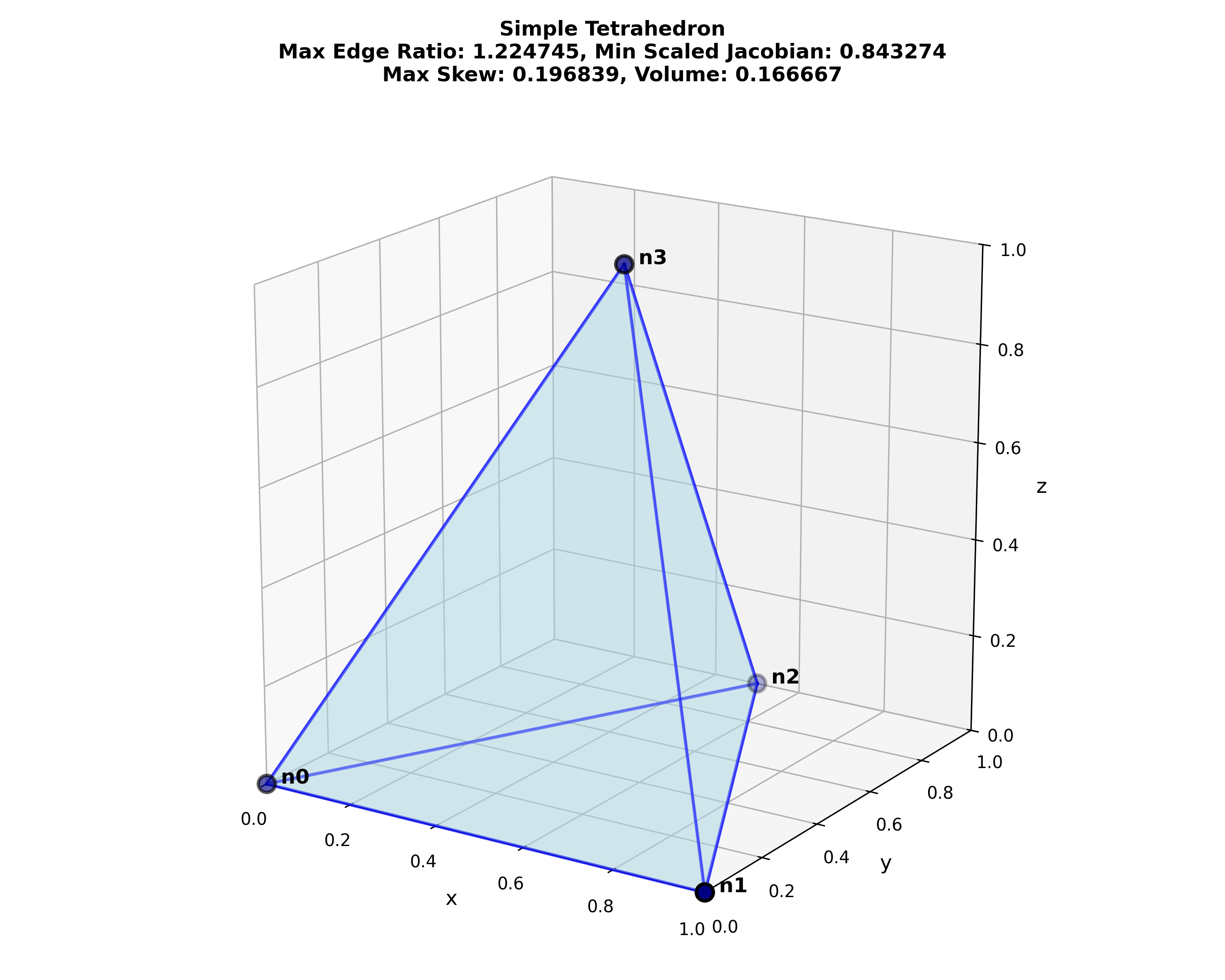
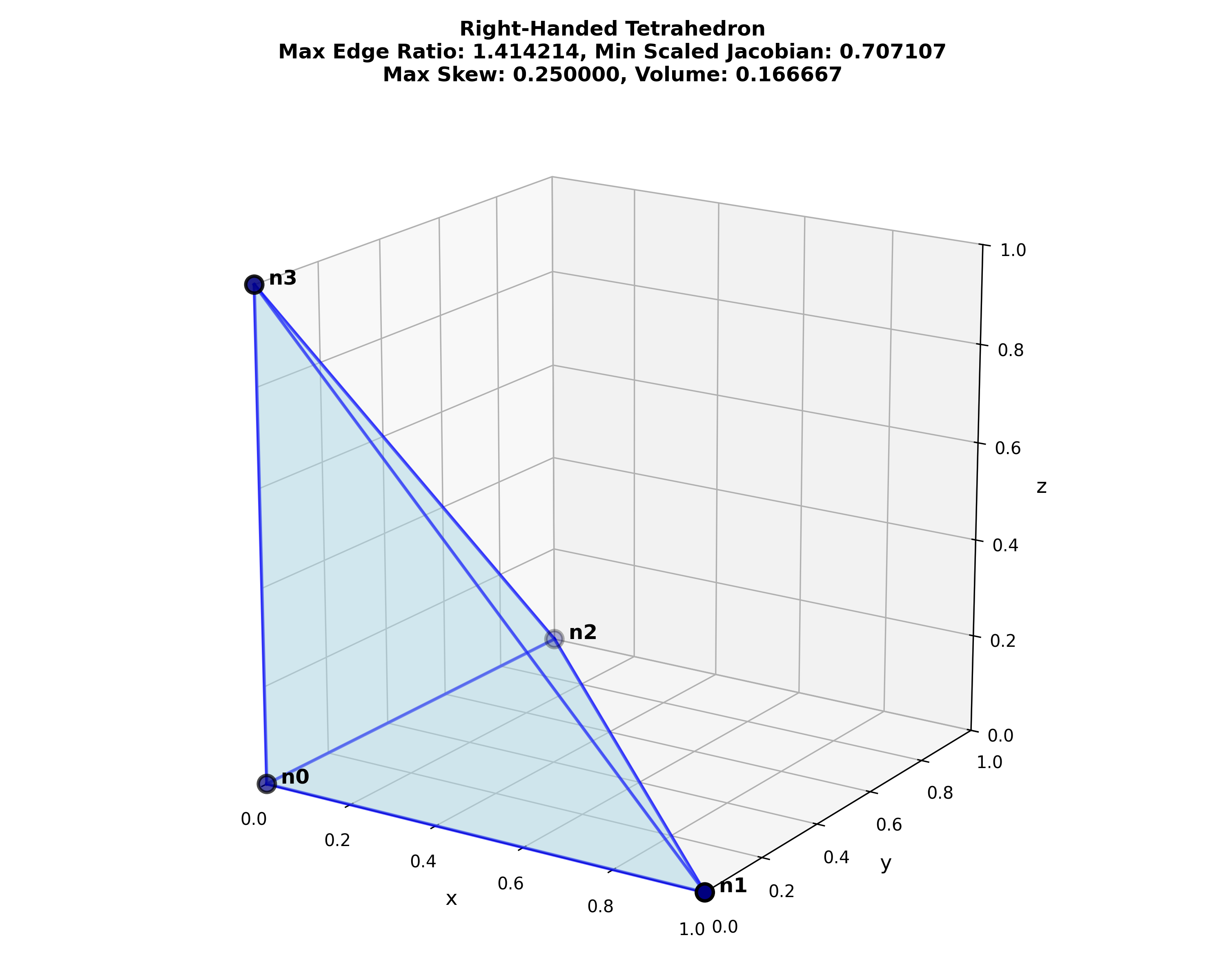
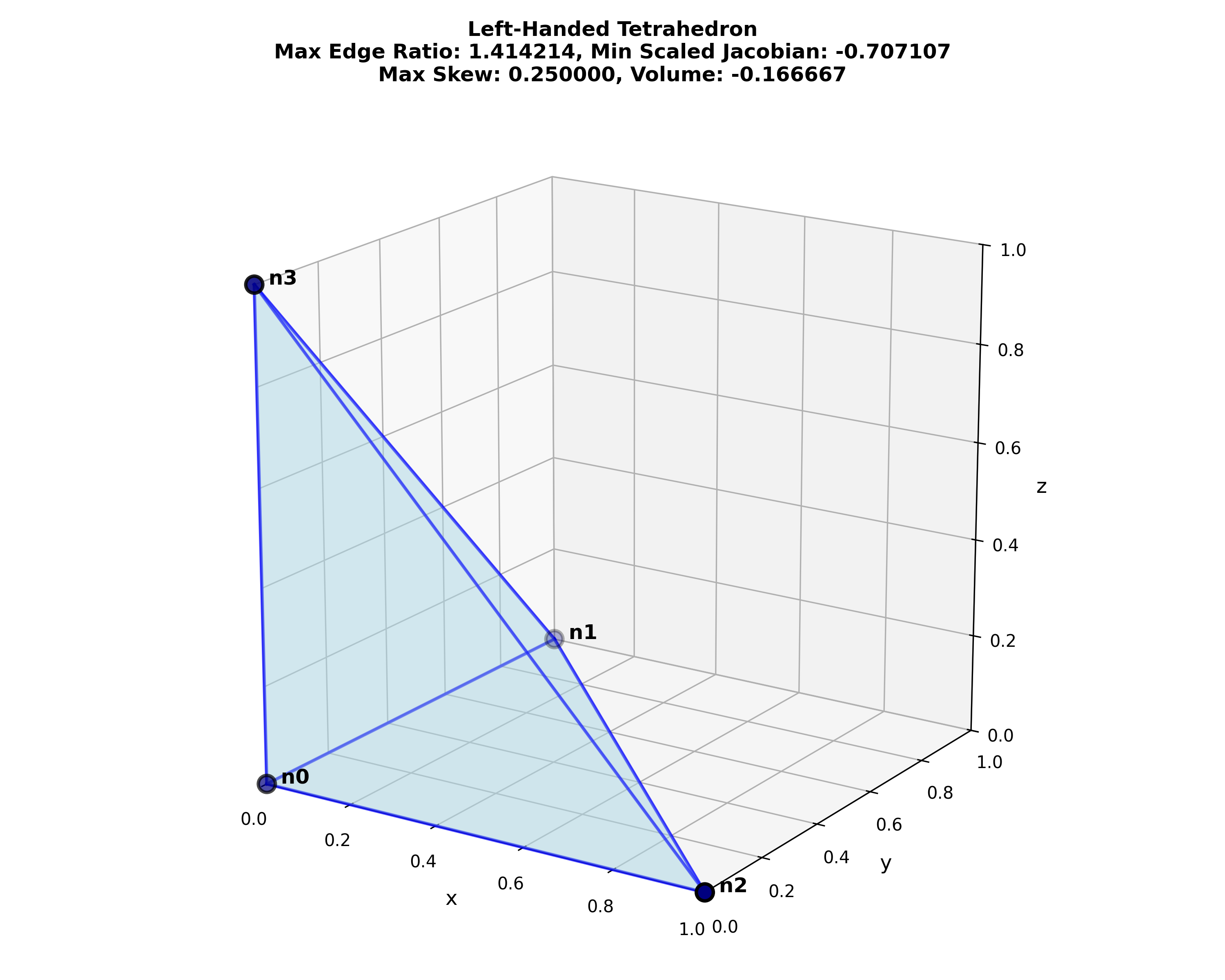
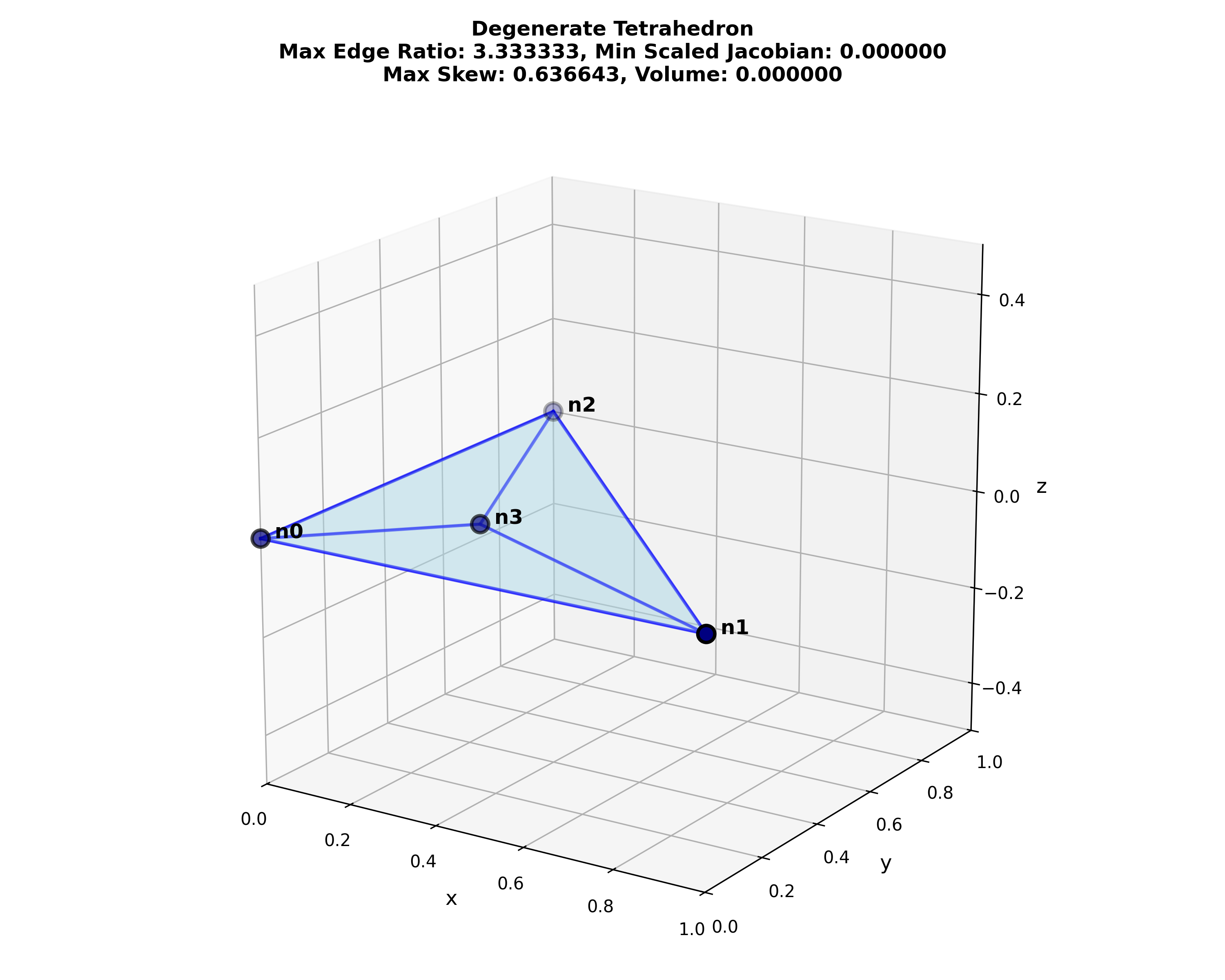
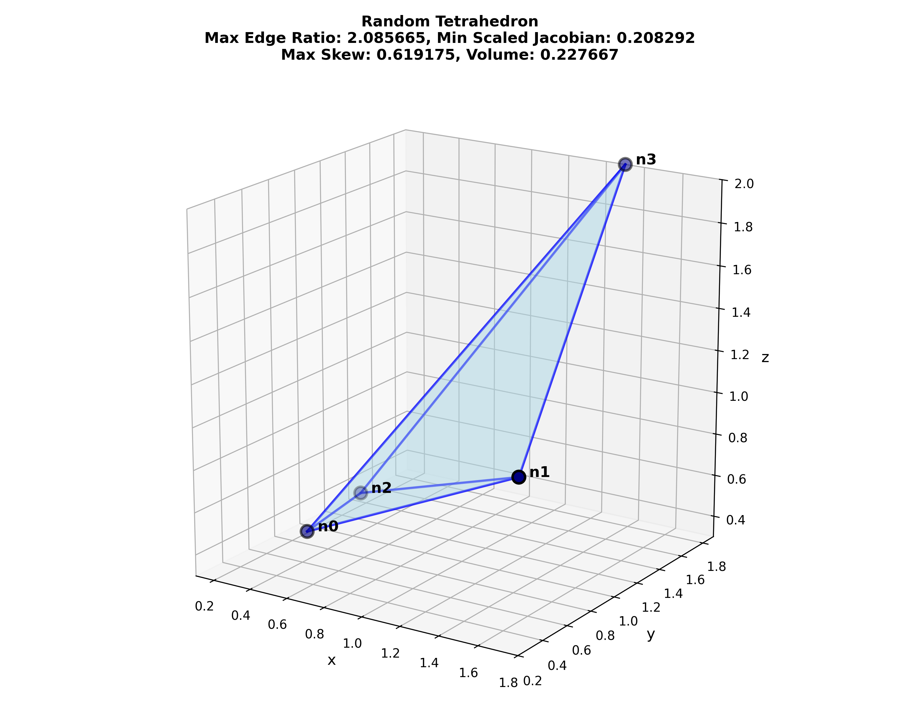
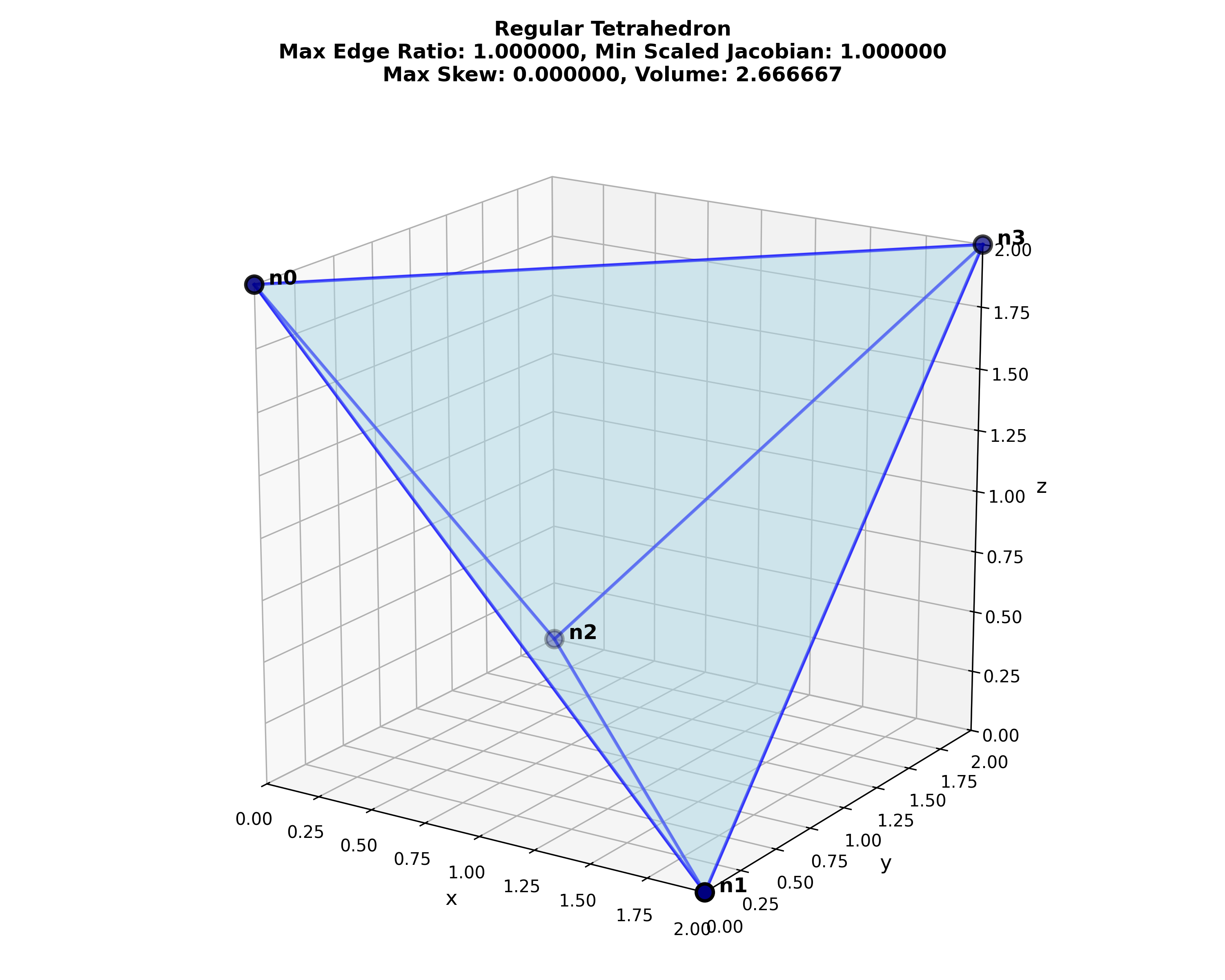
Figure 13-2: Python visualization of the tetrahedron test cases, created with metrics_tetrahedral.py.
Local Numbering Scheme
Nodes
The local numbering scheme for nodes of a tetrahedral element:
        3
       /|\
 L3   / | \  L5
     /  |  \
    0---|---2  (horizontal line is L2)
     \  |  /
  L0  \ | / L1
       \|/
        1

        (vertical line is L4)

where

    L0 = p1 - p0        L3 = p3 - p0
    L1 = p2 - p1        L4 = p3 - p1
    L3 = p0 - p2        L5 = p3 - p2
| node | connected nodes |
|---|---|
| 0 | 1, 2, 3 |
| 1 | 0, 2, 3 |
| 2 | 0, 1, 3 |
| 3 | 0, 1, 2 |
Faces
A tetrahedron has four triangular faces. The faces are typically numbered opposite to the node they do not contain (e.g., face 0 is opposite to node 0).
From the exterior of the element, view the (0, 1, 3) face and unwarp the remaining faces; the four face normals now point out out of the page. The local numbering scheme for faces of a tetrahedral element:
    2-------3-------2
     \  1  / \  0  /
      \   /   \   /
       \ /  2  \ /
        0-------1
         \  3  /
          \   /
           \ /
            2
| face | nodes |
|---|---|
| 0 | 1, 2, 3 |
| 1 | 0, 2, 3 |
| 2 | 0, 1, 3 |
| 3 | 0, 1, 2 |
Source
metrics_tetrahedral.py
metrics_tetrahedral.py
"""Visualize various tetrahedra and calculate quality metrics."""

import numpy as np
import matplotlib.pyplot as plt
from mpl_toolkits.mplot3d.art3d import Poly3DCollection
from typing import List, Tuple


def calculate_edge_vectors(nodes: np.ndarray) -> List[np.ndarray]:
    """Calculate the six edge vectors of a tetrahedron.

    Args:
        nodes (np.ndarray): A 2D numpy array of shape (4, 3)
                            representing the coordinates of the four nodes
                            of the tetrahedron.

    Returns:
        List[np.ndarray]: A list containing six 1D numpy arrays, each
                          representing an edge vector.
    """
    # Base edges (in a cycle 0 -> 1 -> 2 -> 0)
    e0 = nodes[1] - nodes[0]  # n1 - n0
    e1 = nodes[2] - nodes[1]  # n2 - n1
    e2 = nodes[0] - nodes[2]  # n0 - n2

    # Edges connecting the apex (node 3)
    e3 = nodes[3] - nodes[0]  # n3 - n0
    e4 = nodes[3] - nodes[1]  # n3 - n1
    e5 = nodes[3] - nodes[2]  # n3 - n2

    return [e0, e1, e2, e3, e4, e5]


def signed_element_volume(nodes: np.ndarray) -> float:
    """Calculate the signed volume of a tetrahedron.

    Args:
        nodes (np.ndarray): A 2D numpy array of shape (4, 3)
                            representing the coordinates of the four nodes
                            of the tetrahedron.

    Returns:
        float: The signed volume of the tetrahedron.
    """
    v0, v1, v2, v3 = nodes
    return np.dot(np.cross(v1 - v0, v2 - v0), v3 - v0) / 6.0


def maximum_edge_ratio(nodes: np.ndarray) -> float:
    """Calculate the maximum edge ratio (max_length / min_length) of a tetrahedron.

    Args:
        nodes (np.ndarray): A 2D numpy array of shape (4, 3)
                            representing the coordinates of the four nodes
                            of the tetrahedron.

    Returns:
        float: The maximum edge ratio. Returns `float('inf')` if the minimum
               edge length is zero.
    """
    edge_vectors = calculate_edge_vectors(nodes)
    lengths = [np.linalg.norm(v) for v in edge_vectors]
    min_length = min(lengths)
    max_length = max(lengths)
    if min_length == 0:
        return float("inf")
    return float(max_length / min_length)


def minimum_scaled_jacobian(nodes: np.ndarray) -> float:
    """Calculate the minimum scaled Jacobian quality metric for a tetrahedron.

    Args:
        nodes (np.ndarray): A 2D numpy array of shape (4, 3)
                            representing the coordinates of the four nodes
                            of the tetrahedron.

    Returns:
        float: The minimum scaled Jacobian value. Returns 0.0 if the maximum
               nodal Jacobian is zero.
    """
    # The element Jacobian j is 6.0 times the signed element volume
    j = signed_element_volume(nodes) * 6.0

    # Get all six edge lengths
    edge_vectors = calculate_edge_vectors(nodes)
    els = [np.linalg.norm(v) for v in edge_vectors]

    # Compute the four nodal Jacobians
    lambda_0 = els[0] * els[2] * els[3]
    lambda_1 = els[0] * els[1] * els[4]
    lambda_2 = els[1] * els[2] * els[5]
    lambda_3 = els[3] * els[4] * els[5]

    # Find the maximum of the nodal Jacobians (including the element Jacobian)
    lambda_max = max([j, lambda_0, lambda_1, lambda_2, lambda_3])

    # Calculate the final quality metric
    if lambda_max == 0.0:
        return 0.0  # Avoid division by zero for collapsed elements
    else:
        return j * np.sqrt(2.0) / lambda_max


def face_minimum_angle(
    nodes: np.ndarray, n0_idx: int, n1_idx: int, n2_idx: int
) -> float:
    """Calculate the minimum angle of a triangular face.

    Args:
        nodes (np.ndarray): A 2D numpy array of shape (4, 3)
                            representing the coordinates of the four nodes
                            of the tetrahedron.
        n0_idx (int): Index of the first node of the face.
        n1_idx (int): Index of the second node of the face.
        n2_idx (int): Index of the third node of the face.

    Returns:
        float: The minimum angle (in radians) of the triangular face.
    """
    v0 = nodes[n0_idx]
    v1 = nodes[n1_idx]
    v2 = nodes[n2_idx]

    l0 = v2 - v1
    l1 = v0 - v2
    l2 = v1 - v0

    # Normalize
    l0 = l0 / np.linalg.norm(l0)
    l1 = l1 / np.linalg.norm(l1)
    l2 = l2 / np.linalg.norm(l2)

    flip = -1.0
    angles = [
        np.arccos(np.clip(np.dot(l0 * flip, l1), -1.0, 1.0)),
        np.arccos(np.clip(np.dot(l1 * flip, l2), -1.0, 1.0)),
        np.arccos(np.clip(np.dot(l2 * flip, l0), -1.0, 1.0)),
    ]

    return min(angles)


def face_maximum_skew(
    nodes: np.ndarray, n0_idx: int, n1_idx: int, n2_idx: int
) -> float:
    """Calculate the maximum skew for a single triangular face of a tetrahedron.

    Args:
        nodes (np.ndarray): A 2D numpy array of shape (4, 3)
                            representing the coordinates of the four nodes
                            of the tetrahedron.
        n0_idx (int): Index of the first node of the face.
        n1_idx (int): Index of the second node of the face.
        n2_idx (int): Index of the third node of the face.

    Returns:
        float: The maximum skew value for the triangular face.
    """
    tolerance = 1e-9
    equilateral_rad = np.pi / 3.0  # 60 degrees in radians
    minimum_angle = face_minimum_angle(nodes, n0_idx, n1_idx, n2_idx)

    if abs(equilateral_rad - minimum_angle) < tolerance:
        return 0.0
    else:
        return (equilateral_rad - minimum_angle) / equilateral_rad


def maximum_skew(nodes: np.ndarray) -> float:
    """Calculate the maximum skew across all four faces of the tetrahedron.

    Args:
        nodes (np.ndarray): A 2D numpy array of shape (4, 3)
                            representing the coordinates of the four nodes
                            of the tetrahedron.

    Returns:
        float: The maximum skew value among all faces of the tetrahedron.
    """
    # A tetrahedron has four faces, so calculate the skew for each and
    # then take the maximum
    skews = [
        face_maximum_skew(nodes, 0, 1, 2),
        face_maximum_skew(nodes, 0, 1, 3),
        face_maximum_skew(nodes, 0, 2, 3),
        face_maximum_skew(nodes, 1, 2, 3),
    ]

    return max(skews)


def visualize_tetrahedron(
    nodes: np.ndarray,
    title: str = "Tetrahedron",
    show_edges: bool = True,
    show_labels: bool = True,
    save_figure: bool = False,
) -> Tuple[plt.Figure, plt.Axes]:
    """Visualize a tetrahedron given its four node coordinates and display quality metrics.

    Args:
        nodes (np.ndarray): A 2D numpy array of shape (4, 3)
                            representing the coordinates of the four nodes
                            of the tetrahedron.
        title (str, optional): Title for the plot. Defaults to "Tetrahedron".
        show_edges (bool, optional): Whether to display the edges of the tetrahedron.
                                     Defaults to True.
        show_labels (bool, optional): Whether to display labels for the nodes.
                                      Defaults to True.
        save_figure (bool, optional): Whether to save the figure as a PNG file.
                                      Defaults to False.

    Returns:
        Tuple[plt.Figure, plt.Axes]: A tuple containing the matplotlib Figure and Axes objects.
    """
    nodes = np.array(nodes)

    fig = plt.figure(figsize=(10, 8))
    ax = fig.add_subplot(111, projection="3d")

    # Define the four faces of the tetrahedron
    # Each face is a triangle defined by three nodes
    faces = [
        [nodes[0], nodes[1], nodes[2]],  # Face 0-1-2
        [nodes[0], nodes[1], nodes[3]],  # Face 0-1-3
        [nodes[0], nodes[2], nodes[3]],  # Face 0-2-3
        [nodes[1], nodes[2], nodes[3]],  # Face 1-2-3
    ]

    # Create the 3D polygon collection for faces
    face_collection = Poly3DCollection(
        faces, alpha=0.3, facecolor="lightblue", edgecolor="blue", linewidths=1.5
    )
    ax.add_collection3d(face_collection)

    # Plot nodes
    ax.scatter(
        nodes[:, 0],
        nodes[:, 1],
        nodes[:, 2],
        c="navy",
        s=100,
        marker="o",
        edgecolors="black",
        linewidths=2,
    )

    # Add node labels
    if show_labels:
        for i, node in enumerate(nodes):
            ax.text(
                node[0], node[1], node[2], f"  n{i}", fontsize=12, fontweight="bold"
            )

    # Draw edges if requested
    if show_edges:
        edges = [
            (0, 1),
            (1, 2),
            (2, 0),  # Base triangle
            (0, 3),
            (1, 3),
            (2, 3),  # Edges to apex
        ]
        for edge in edges:
            points = nodes[list(edge)]
            ax.plot3D(*points.T, "b-", linewidth=2, alpha=0.6)

    # Calculate all metrics
    volume = signed_element_volume(nodes)
    max_edge_ratio = maximum_edge_ratio(nodes)
    min_scaled_jac = minimum_scaled_jacobian(nodes)
    max_skew = maximum_skew(nodes)

    # Set labels and title
    ax.set_xlabel("x", fontsize=12)
    ax.set_ylabel("y", fontsize=12)
    ax.set_zlabel("z", fontsize=12)

    title_text = f"{title}\n"
    title_text += f"Max Edge Ratio: {max_edge_ratio:.6f}, "
    title_text += f"Min Scaled Jacobian: {min_scaled_jac:.6f}\n"
    title_text += f"Max Skew: {max_skew:.6f}, "
    title_text += f"Volume: {volume:.6f}"

    ax.set_title(title_text, fontsize=12, fontweight="bold")

    # Set equal aspect ratio
    max_range = (
        np.array(
            [
                nodes[:, 0].max() - nodes[:, 0].min(),
                nodes[:, 1].max() - nodes[:, 1].min(),
                nodes[:, 2].max() - nodes[:, 2].min(),
            ]
        ).max()
        / 2.0
    )

    mid_x = (nodes[:, 0].max() + nodes[:, 0].min()) * 0.5
    mid_y = (nodes[:, 1].max() + nodes[:, 1].min()) * 0.5
    mid_z = (nodes[:, 2].max() + nodes[:, 2].min()) * 0.5

    ax.set_xlim(mid_x - max_range, mid_x + max_range)
    ax.set_ylim(mid_y - max_range, mid_y + max_range)
    ax.set_zlim(mid_z - max_range, mid_z + max_range)

    # ax.view_init(elev=63, azim=-110, roll=0)
    ax.view_init(elev=18, azim=-57, roll=0)
    ax.set_aspect("equal")
    plt.tight_layout()

    if save_figure:
        filename = title.replace(" ", "_").lower() + ".png"
        plt.savefig(filename, dpi=300)
        print(f"Saved figure to {filename}")

    return fig, ax


# Example 1: Simple tetrahedron
NAME = "Simple Tetrahedron"
print(f"Example 1: {NAME}")
nodes_1 = np.array(
    [
        [0.0, 0.0, 0.0],
        [1.0, 0.0, 0.0],
        [0.5, 1.0, 0.0],
        [0.5, 0.5, 1.0],
    ]
)
visualize_tetrahedron(nodes_1, NAME, save_figure=True)

# Example 2: Positive signed volume (right-handed)
NAME = "Right-Handed Tetrahedron"
print(f"\nExample 2: {NAME}")
nodes_2 = np.array(
    [
        [0.0, 0.0, 0.0],
        [1.0, 0.0, 0.0],
        [0.0, 1.0, 0.0],
        [0.0, 0.0, 1.0],
    ]
)
visualize_tetrahedron(nodes_2, NAME, save_figure=True)

# Example 3: Negative signed volume (left-handed / inverted)
NAME = "Left-Handed Tetrahedron"
print(f"\nExample 3: {NAME}")
nodes_3 = np.array(
    [
        [0.0, 0.0, 0.0],
        [1.0, 0.0, 0.0],  # Node 1
        [0.0, 1.0, 0.0],  # Node 2
        [0.0, 0.0, 1.0],  # Node 3
    ]
)
# Connectivity is [0, 2, 1, 3] - swapped nodes 1 and 2
nodes_3_inverted = nodes_3[[0, 2, 1, 3]]
visualize_tetrahedron(nodes_3_inverted, NAME, save_figure=True)

# Example 4: Degenerate tetrahedron (zero volume)
NAME = "Degenerate Tetrahedron"
print(f"\nExample 4: {NAME}")
nodes_4 = np.array(
    [
        [0.0, 0.0, 0.0],
        [1.0, 0.0, 0.0],
        [0.0, 1.0, 0.0],
        [0.3, 0.3, 0.0],  # Co-planar with other nodes
    ]
)
visualize_tetrahedron(nodes_4, NAME, save_figure=True)

# Example 5: Random tetrahedron
NAME = "Random Tetrahedron"
print(f"\nExample 5: {NAME}")
nodes_5 = np.array(
    [
        [0.5, 0.5, 0.5],
        [1.8, 0.2, 1.1],
        [0.1, 1.5, 0.3],
        [1.3, 1.9, 2.0],
    ]
)
visualize_tetrahedron(nodes_5, NAME, save_figure=True)

# Example 6: Regular tetrahedron (for maximum skew test, has zero skew)
NAME = "Regular Tetrahedron"
print(f"\nExample 6: {NAME}")
nodes_6 = np.array(
    [
        [0.0, 0.0, 2.0],
        [2.0, 0.0, 0.0],
        [0.0, 2.0, 0.0],
        [2.0, 2.0, 2.0],
    ]
)
visualize_tetrahedron(nodes_6, NAME, save_figure=True)

plt.show()
References
-
Knupp PM, Ernst CD, Thompson DC, Stimpson CJ, Pebay PP. The verdict geometric quality library. SAND2007-1751. Sandia National Laboratories (SNL), Albuquerque, NM, and Livermore, CA (United States); 2006 Mar 1. link ↩ ↩2 ↩3 ↩4 ↩5 ↩6
Triangular Metrics
automesh metrics tri --help
automesh implements the following triangular element quality metrics1:
- Maximum edge ratio
- Minimum scaled Jacobian
- Maximum skew
- Element area
- Minimum angle
A brief description of each metric follows.
Maximum Edge Ratio
- measures the ratio of the longest edge to the shortest edge in a mesh element.
- A ratio of 1.0 indicates perfect element quality, whereas a very large ratio indicates bad element quality.
- Knupp et al.1 (page 26) indicate an acceptable range of
[1.0, 1.3].
Minimum Scaled Jacobian
- evaluates the determinant of the Jacobian matrix at each of the corners nodes, normalized by the corresponding edge lengths, and returns the minimum value of those evaluations.
- Knupp et al.1 (page 29) indicate an acceptable range of
[0.5, 2*sqrt(3)/3][0.5, 1.2]. - A scaled Jacobian close to
0indicates that the triangle is poorly shaped (e.g., very thin or degenerate), which can lead to numerical instability. - A scaled Jacobian of
1indicates that the triangle is equilateral, which is the ideal shape for numerical methods. This is achieved through scaling as follows:
- In the preceding equation,
- is the smallest angle of an equilateral triangle, and
- is the smallest angle of the subject triangle.
Maximum Skew
- Skew measures how much an element deviates from being a regular shape (e.g., in 3D a cube or a regular tetrahedron; in 2D a square or equilateral triangle). A skew value of 0 indicates a perfectly regular shape, while higher values indicate increasing levels of distortion.
- Knupp et al.1 does not give a definition of skew for triangles, so we provide our definition below. For a triangle where is the smallest angle of the triangle,
- For an equilateral triangle, and .
- In the limit as .
Element Area
- Measures the area of the element.
Minimum Angle
- The smallest the three angles of a triangle.
- Ideal value: (for an equilateral triangle).
- The should be maximized (kept as close to as possible) and above a minimum threshold (e.g., to ).
- Acute angles (close to ) cause high errors and numerical instability.
Unit Tests
We use the ABAQUS input file single_valence_04_noise2.inp.
We import the file into Cubit and create a triangular surface mesh:
import abaqus mesh geometry  "/Users/chovey/autotwin/automesh/tests/input/single_valence_04_noise2.inp" feature_angle 135.00
surface 1 scheme trimesh minimum size 100
surface 2 scheme trimesh minimum size 100
surface 3 scheme trimesh minimum size 100
surface 4 scheme trimesh minimum size 100
surface 5 scheme trimesh minimum size 100
# surface 6 scheme trimesh minimum size 100 # there is no side 6, two sides were merged
delete mesh surface all propagate
surface all scheme trimesh
mesh surface all
quality tri all aspect ratio global draw mesh list detail
quality tri all scaled jacobian global draw mesh list detail
quality tri all element area global draw mesh list detail
export stl ascii "/Users/chovey/autotwin/automesh/tests/input/single_valence_04_noise2.stl" mesh  overwrite
We also examine several .stl files and process them, for example,
import stl "/Users/chovey/autotwin/automesh/tests/input/one_facet.stl" feature_angle 135.00 merge make_elements
surface 1 scheme trimesh minimum size 100
delete mesh surface 1  propagate
surface 1  scheme trimesh
mesh surface 1
quality tri all aspect ratio global draw mesh list detail
quality tri all scaled jacobian global draw mesh list detail
quality tri all element area global draw mesh list detail
We verify the following element qualities:
| file | e | area | (deg) | |||
|---|---|---|---|---|---|---|
A | 1 | 1.508 [1.508] | 0.761 [0.761] | 0.313 [0.331] | 0.610 [0.610] | 41.2 [41.2] |
A | 2 | 1.550 [1.550] | 0.739 [0.739] | 0.337 [0.337] | 0.550 [0.550] | 39.8 [39.8] |
A | 3 | 1.787 [1.787] | 0.639 [0.639] | 0.440 [0.440] | 0.569 [0.569] | 33.6 [33.6] |
A | 4 | 1.915 [1.915] | 0.595 [0.595] | 0.483 [0.483] | 0.402 [0.402] | 31.0 [31.0] |
A | 5 | 2.230 [2.230] | 0.426 [0.426] | 0.639 [0.639] | 0.342 [0.342] | 21.7 [21.7] |
A | 6 | 1.623 [1.623] | 0.700 [0.700] | 0.378 [0.378] | 0.571 [0.571] | 37.3 [37.1] |
A | 7 | 1.240 [1.240] | 0.898 [0.898] | 0.149 [0.149] | 0.424 [0.424] | 51.0 [51.0] |
A | 8 | 1.385 [1.385] | 0.831 [0.831] | 0.233 [0.233] | 0.443 [0.443] | 46.1 [46.1] |
A | 9 | 1.606 [1.606] | 0.719 [0.719] | 0.358 [0.358] | 0.648 [0.648] | 38.5 [38.5] |
A | 10 | 1.429 [1.429] | 0.806 [0.806] | 0.262 [0.262] | 0.704 [0.704] | 44.3 [44.3] |
A | 11 | 1.275 [1.275] | 0.880 [0.880] | 0.172 [0.172] | 0.668 [0.668] | 49.7 [49.7] |
A | 12 | 1.436 [1.436] | 0.804 [0.804] | 0.264 [0.264] | 0.516 [0.516] | 44.1 [44.1] |
B | 1 | 1.414 [1.414] | 0.816 [0.816] | 0.250 [0.250] | 0.500 [0.500] | 45.0 [45.0] |
C | 1 | 1.000 [1.000] | 1.000 [1.000] | 0.000 [0.000] | 6.928 [6.928] | 60.0 [60.0] |
D | 1 | 1.000 [1.000] | 1.000 [1.000] | 0.000 [0.000] | 0.433 [0.433] | 60.0 [60.0] |
E | 1 | 1.256 [1.256] | 0.869 [0.869] | 0.187 [0.187] | 3.273 [3.273] | 48.8 [48.8] |
Figure 14-1: Triangle metrics.
Leading values are from automesh.
Values in [brackets] are from an independent Python calculation, (see metrics_triangular.py) and agree with automesh in double precision with a tolerance of less than 2.22e-15.
Except for edge ratio, all values were also verified with Cubit.
Cubit uses the term Aspect Ratio; it is not the same as Edge Ratio.
- File
Aissingle_valence_04_noise2.inp. - File
Bisone_facet.stl. - File
Cis an equilateral triangle with nodal coordinates at(-2, 0, 0),(2, 0, 0), and(0, 2*sqrt(3), 0)and has side length4.0, saved totests/input/equilateral_4.stl. - File
Dis an equilateral triangle with nodal coordinates at(-0.5, 0, 0),(0.5, 0, 0), and(0, sqrt(3) / 2, 0)and has side length1.0, saved totests/input/equilateral_1.stl. - File
Eis an off axis triangle with approximate (30, 60, 90) degree inner angles, with coordinates at(0.0, 1.0, 3.0),(2.0, 0.0, 2.0), and(1.0, sqrt(3.0) + 1.0, 1.0), saved totests/input/off_axis.stl. eis the element number in the mesh.
Local Numbering Scheme
Nodes
The local numbering scheme for nodes of a triangular element:
        2
       / \
      /   \
     /     \
    /       \
   0---------1
| node | connected nodes |
|---|---|
| 0 | 1, 2 |
| 1 | 0, 2 |
| 2 | 0, 1 |
Faces
The local numbering scheme for faces of a triangular element:
| face | nodes |
|---|---|
| 0 | 0, 1, 2 |
Source
metrics_triangular.py
metrics_triangular.py
"""This script is a quality control tool for the metrics of a tri mesh."""

from typing import Final

import numpy as np

DEG_TO_RAD: Final[float] = np.pi / 180.0
J_EQUILATERAL: Final[float] = np.sqrt(3.0) / 2.0  # sin(60 deg)


def nf(x):
    """Does a list comprehension, casting each item from a np.float64
    to a float."""
    return [float(y) for y in x]


nodal_coordinates = (
    (-0.2, 1.2, -0.1),  # single_valence_04_noise2.inp begin
    (1.180501, 0.39199, 0.3254445),
    (0.1, 0.2, 0.3),
    (-0.001, -0.021, 1.002),
    (1.2, -0.1, 1.1),
    (1.03, 1.102, -0.25),
    (0.0, 1.0, 1.0),
    (1.01, 1.02, 1.03),  # single_valence_04_noise2.inp end
    (0.0, 0.0, 1.0),  # one_facet.stl begin
    (0.0, 0.0, 0.0),
    (1.0, 0.0, 0.0),  # one_facet.stl end
    (-2.0, 0.0, 0.0),  # equilateral with edge length 4.0 start
    (2.0, 0.0, 0.0),
    (0.0, 2.0 * np.sqrt(3.0), 0.0),  # equilateral with edge length 4.0 end
    (-0.5, 0.0, 0.0),  # equilateral with edge length 1.0 start
    (0.5, 0.0, 0.0),
    (0.0, np.sqrt(3.0) / 2.0, 0.0),  # equilateral with edge length 1.0 end
    (0.0, 1.0, 3.0),  # off_axis.stl begin
    (2.0, 0.0, 2.0),
    (1.0, np.sqrt(3.0) + 1.0, 1.0),  # off_axis.stl end
)

element_node_connectivity = (
    (1, 2, 3),  # single_valence_04_noise2.inp begin
    (4, 2, 5),
    (1, 6, 2),
    (4, 3, 2),
    (4, 1, 3),
    (4, 7, 1),
    (2, 8, 5),
    (6, 8, 2),
    (7, 8, 6),
    (1, 7, 6),
    (4, 5, 8),
    (7, 4, 8),  # single_valence_04_noise2.inp end
    (9, 10, 11),  # one_facet.stl
    (12, 13, 14),  # equilateral triangle with side length 4.0
    (15, 16, 17),  # equilateral triangle with side length 1.0
    (18, 19, 20),  # off_axis.stl
)

NODE_NUMBERING_OFFSET: Final[int] = 1

mesh_element_max_edge_lengths = []
mesh_element_edge_ratios = []
mesh_element_minimum_angles = []
mesh_element_maximum_skews = []
mesh_element_areas = []
mesh_element_jacobians = []
mesh_element_jacobians_scaled = []


def angle(a: np.ndarray, b: np.ndarray) -> float:
    """Given two vectors, find the angle between them."""
    dot_product = np.dot(a, b)
    norm_a = np.linalg.norm(a)
    norm_b = np.linalg.norm(b)

    cos_theta = dot_product / (norm_a * norm_b)

    angle_radians = np.arccos(cos_theta)
    result = np.degrees(angle_radians)  # degrees

    return result


for element in element_node_connectivity:
    print(f"element with nodes: {element}")
    path = element + (element[0],)
    # print(f"  node path {path}")
    pairs = tuple(zip(element, element[1:] + (element[0],)))
    print(f"  node pairs {pairs}")
    element_edge_ratios = []
    element_minimum_angles = []
    element_minimum_jacobians = []
    edge_vectors = ()
    # edge ratios
    for pair in pairs:
        print(f"    pair {pair}")
        aa, bb = pair
        edge = np.array(nodal_coordinates[bb - NODE_NUMBERING_OFFSET]) - np.array(
            nodal_coordinates[aa - NODE_NUMBERING_OFFSET]
        )
        edge_vectors = edge_vectors + (edge,)
        edge_length = np.linalg.norm(edge)
        # print(f"    lens {edge_length}")
        element_edge_ratios.append(edge_length)

    # print(f"  edge ratios {element_edge_ratios}")

    # edge ratios
    len_max = max(element_edge_ratios)
    # print(f"  max edge ratio {len_max}")
    mesh_element_max_edge_lengths.append(len_max)

    len_min = min(element_edge_ratios)
    # print(f"  min edge ratio {len_min}")
    ratio = len_max / len_min
    mesh_element_edge_ratios.append(ratio)

    # edge vectors and then angles
    edge_vectors_pairs = tuple(zip(edge_vectors, edge_vectors[1:] + (edge_vectors[0],)))
    # print(f"  edge vectors pairs {edge_vectors_pairs}")

    for item in edge_vectors_pairs:
        # print(f"    edge vectors pair {item}")
        # flip the direction of the first vector so that it shares an origin
        # with the second vector
        angle_degrees = angle(-1.0 * item[0], item[1])
        # print(f"    angle {angle_degrees}")
        element_minimum_angles.append(angle_degrees)

    print(f"  element angles (deg) {nf(element_minimum_angles)}")
    angle_min = min(element_minimum_angles)
    print(f"  min angle (deg) {angle_min}")
    mesh_element_minimum_angles.append(angle_min)

    jacobian_e = np.sin(angle_min * DEG_TO_RAD)
    jacobian_scaled_e = jacobian_e / J_EQUILATERAL
    print(f"  min Jacobian (sin(angle_min)) {jacobian_e}")
    print(f"  min scaled Jacobian  {jacobian_scaled_e}")
    mesh_element_jacobians.append(jacobian_e)
    mesh_element_jacobians_scaled.append(jacobian_scaled_e)

    skew_max = (60.0 - angle_min) / 60.0
    mesh_element_maximum_skews.append(skew_max)

    # Compute areas only for triangles for now.
    if len(element) == 3:
        # area of a triangle
        aa = np.linalg.norm(edge_vectors[0])
        bb = np.linalg.norm(edge_vectors[1])
        cc = np.linalg.norm(edge_vectors[2])
        # Calculate the semi-perimeter
        ss = (aa + bb + cc) / 2.0
        # Use Heron's formula to calculate the area
        area = np.sqrt(ss * (ss - aa) * (ss - bb) * (ss - cc))
        mesh_element_areas.append(area)

print(f"\nmesh element max edge lengths: {nf(mesh_element_max_edge_lengths)}")
print(f"\nmesh element edge ratios: {nf(mesh_element_edge_ratios)}")
print(f"\nmesh element minimum angles: {nf(mesh_element_minimum_angles)}")
print(f"\nmesh element maximum skews: {nf(mesh_element_maximum_skews)}")
print(f"\nmesh element areas: {nf(mesh_element_areas)}")
print(f"\nmesh minimum scaled Jacobians: {nf(mesh_element_jacobians_scaled)}")
References
-
Knupp PM, Ernst CD, Thompson DC, Stimpson CJ, Pebay PP. The verdict geometric quality library. SAND2007-1751. Sandia National Laboratories (SNL), Albuquerque, NM, and Livermore, CA (United States); 2006 Mar 1. link ↩ ↩2 ↩3 ↩4
Development


Prerequisites
-
Rust and Cargo, installed via Rustup:
curl --proto '=https' --tlsv1.2 -sSf https://sh.rustup.rs | shRust updates occur every six weeks. To update Rust:
rustup update
Optional
-
VS Code with the following extensions:
-
cargo bibuild+install helper (macOS) —scripts/cargo-bichainscargo buildandcargo install --path . --forceinto one command; see Development Cycle Overview for why that matters. Install it once, symlinked so future updates to the script are picked up automatically:ln -s "$(pwd)/scripts/cargo-bi" ~/.cargo/bin/cargo-bi ln -s "$(pwd)/scripts/cargo-bi-nightly" ~/.cargo/bin/cargo-bi-nightlyCargo's plugin mechanism treats any executable named
cargo-*onPATHas the subcommandcargo *, so this makescargo bi(andcargo bi --release) available immediately, from any directory containing aCargo.toml.cargo bi-nightlyis the same helper built and installed with the nightly toolchain instead — a fallback for a branch whoseconspiredependency is pinned to a git rev that needs a Rust feature not yet in your installed stable toolchain (rustup update stableis usually the simpler fix; aCargo.tomlcomment on such a branch says which feature and when it stabilized).
Clone Repository
git clone git@github.com:autotwin/automesh.git
cd automesh
Building the Book Locally
The book embeds live command output via mdbook-cmdrun: most pages run
automesh (some piped through ansifilter to strip ANSI color codes for
plain-text embedding), and a few run cat or python. If automesh isn't
resolvable on PATH, mdbook-cmdrun fails silently — the affected output
blocks simply render empty, with no error — so before running mdbook build
or mdbook serve, make sure both are available:
cd automesh               # the repository root, containing Cargo.toml
cargo install --path .    # installs `automesh` to ~/.cargo/bin; re-run after
                          # source changes you want reflected in the book
brew install ansifilter   # macOS, one-time (apt-get install ansifilter on Linux)
cargo install --path . must be run from the repository root (or pass that
path explicitly, e.g. cargo install --path ~/autotwin/automesh from
anywhere) — --path points at the directory containing the crate's
Cargo.toml, not at the book or any other subdirectory.
Both install locations are typically already on PATH via Rustup/Homebrew,
so no PATH changes should be needed.
Development Cycle Overview
- Branch
- Develop
cargo buildcargo install --path . --force— updates theautomeshonPATH(~/.cargo/bin/automesh).cargo buildalone only writes totarget/; plainautomeshkeeps resolving to whatever was last installed until this is rerun.cargo bi(orcargo bi --release) runs both steps in one command — see Optional for one-time setup.
- Develop:
- tests
- implementation
- Document:
mdbook build(see Building the Book Locally for prerequisites)- output:
automesh/book/build
- output:
mdbook serve --open- interactive mode
- On the local machine, with Firefox, open the
index.htmlfile, e.g.,file:///Users/chovey/autotwin/automesh/book/build/index.html
cargo rustdoc --open -- --html-in-header docs/katex.html
- Test:
cargo testcargo run// test without required input and output flagscargo run --release -- -i tests/input/f.npy -o foo.exocargo run -- --help
- Lint:
cargo clippy
- Pre-commit:
pre-commit run --all-files
- Clean:
cargo clean
- Merge Request