Smoothing

Introduction

Both Laplacian smoothing¹ and Taubin smoothing^{2 3} are smoothing operations that adjust the positions of the nodes in a finite element mesh.

Laplacian smoothing, based on the Laplacian operator, computes the average position of a point's neighbors and moves the point toward the average. This reduces high-frequency noise but can result in a loss of shape and detail, with overall shrinkage.

Taubin smoothing is an extension of Laplacian smoothing that seeks to overcome the shrinkage drawback associated with the Laplacian approach. Taubin is a two-pass approach. The first pass smooths the mesh. The second pass re-expands the mesh.

Laplacian Smoothing

Consider a subject node with position $\mathbf{p}=\mathbf{p}(x,y,z)\in {\mathbb{R}}^3$. The subject node connects to $n$ neighbor points ${\mathbf{q}}_i$ for $i\in [1,n]$ through $n$ edges.

For concereteness, consider a node with four neighbors, shown in the figure below.

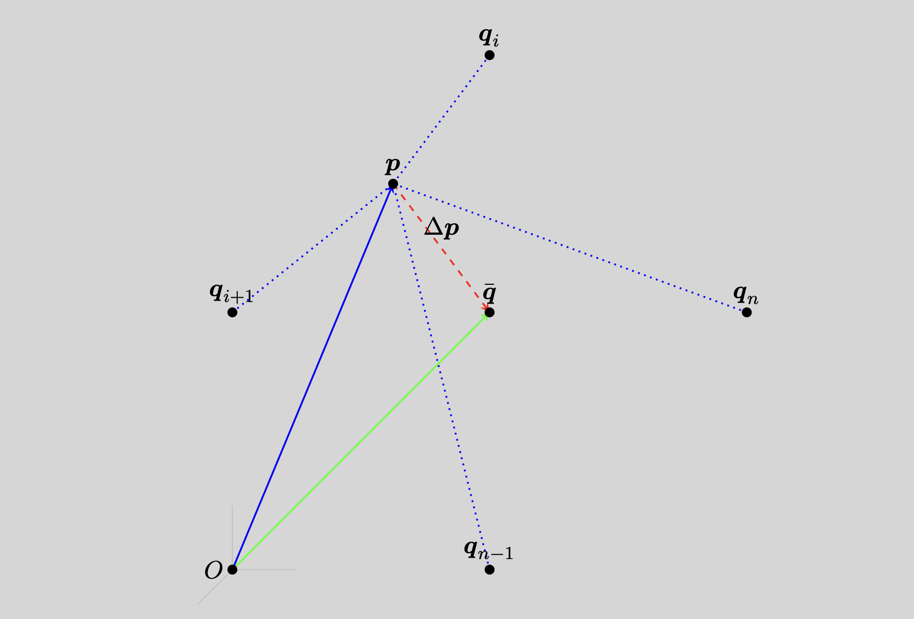
Figure: The subject node $\mathbf{p}$ with edge connections (dotted lines) to neighbor nodes ${\mathbf{q}}_i$ with $i\in [1,n]$ (withouth loss of generality, the specific example of $n=4$ is shown). The average position of all neighbors of $\mathbf{p}$ is denoted $\bar{\mathbf{q}}$, and the gap $\Delta \mathbf{p}$ (dashed line) originates at $\mathbf{p}$ and terminates at $\bar{\mathbf{q}}$.

Define $\bar{\mathbf{q}}$ as the average position of all ${\mathbf{q}}_i$ neighbors of $\mathbf{p}$,

$$\bar{\mathbf{q}}:=\frac{1}{n}\sum _{i=1}^n{\mathbf{q}}_i.$$

Define the gap vector $\Delta \mathbf{p}$ as originating at $\mathbf{p}$ and terminating at $\bar{\mathbf{q}}$ (viz., $\mathbf{p}+\Delta \mathbf{p}=\bar{\mathbf{q}}$),

$$\Delta \mathbf{p}:=\bar{\mathbf{q}}-\mathbf{p}.$$

Let $\lambda \in {\mathbb{R}}^{+}$ be the positive scaling factor for the gap $\Delta \mathbf{p}$.

Since

$$\bar{\mathbf{q}}=\mathbf{p}+\lambda \Delta \mathbf{p}\mathrm{when}\lambda =1,$$

subdivision of this relationship into several substeps gives rise to an iterative approach. We typically select $\lambda <1$ to avoid overshoot of the update, $\lambda \in {\mathbb{R}}^{+}\subset (0,1)$.

At iteration $k$, we update the position of ${\mathbf{p}}^{(k)}$ by an amount $\lambda \Delta {\mathbf{p}}^{(k)}$ to ${\mathbf{p}}^{(k+1)}$ as

$${\mathbf{p}}^{(k+1)}:={\mathbf{p}}^{(k)}+\lambda \Delta {\mathbf{p}}^{(k)},$$

with

$$\Delta {\mathbf{p}}^{(k)}={\bar{\mathbf{q}}}^{(k)}-{\mathbf{p}}^{(k)}.$$

Thus

$${\mathbf{p}}^{(k+1)}:={\mathbf{p}}^{(k)}+\lambda \left(\Delta {\mathbf{p}}^{(k)}\right),$$

$${\mathbf{p}}^{(k+1)}:={\mathbf{p}}^{(k)}+\lambda \left({\bar{\mathbf{q}}}^{(k)}-{\mathbf{p}}^{(k)}\right),$$

and finally

$$\boxed{{\mathbf{p}}^{(k+1)}:={\mathbf{p}}^{(k)}+\lambda \left(\frac{1}{n}\sum _{i=1}^n{\mathbf{q}}_i^{(k)}-{\mathbf{p}}^{(k)}\right).}$$

The formulation above, based on the average position of the neighbors, is a special case of the more generalized presentation of Laplace smoothing, wherein a normalized weighting factor, $w_i$, is used:

$${\mathbf{p}}^{(k+1)}:={\mathbf{p}}^{(k)}+\lambda \sum _{i=1}^n{w}_i\left({\mathbf{q}}_i^{(k)}-{\mathbf{p}}^{(k)}\right).$$

When all weights are equal and normalized by the number of neighbors, $w_i=\frac{1}{n}$, the special case presented in the box above is recovered.

Example

For a 1D configuration, consider a node with initial position $\mathbf{p}=1.5$ with two neighbors (that never move) with positions ${\mathbf{q}}_1=0.0$ and ${\mathbf{q}}_2=1.0$ ($\bar{\mathbf{q}}=0.5$). With $\lambda =0.3$, the table below shows updates for for position $\mathbf{p}$.

Table: Iteration updates of a 1D example.

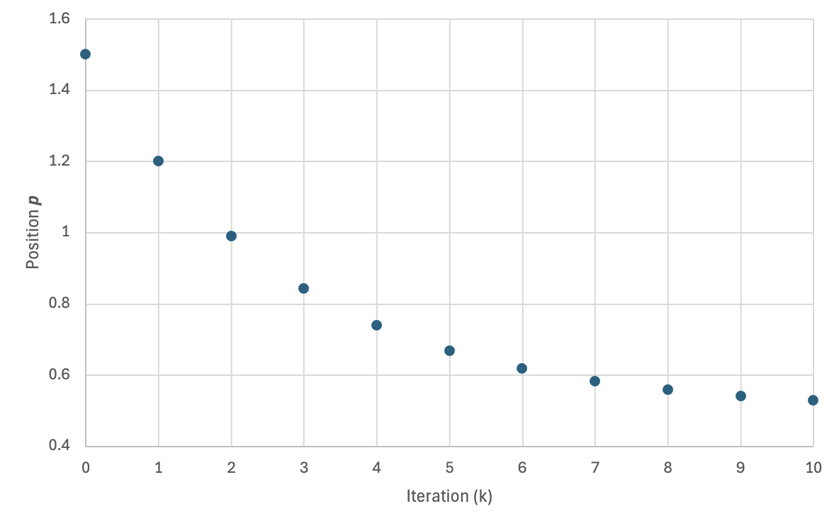
Figure: Convergence of position $\mathbf{p}$ toward $0.5$ as a function of iteration $k$.

Taubin Smoothing

Taubin smoothing is a two-parameter, two-pass iterative variation of Laplace smoothing. Specifically with the definitions used in Laplacian smoothing, a second negative parameter $\mu$ is used, where

$$\mu \in {\mathbb{R}}^{-}\subset (-1,0)\lambda \in {\mathbb{R}}^{+}\subset (0,1)\mathrm{and}\lambda <-\mu .$$

The first parameter, $\lambda$, tends to smooth (and shrink) the domain. The second parameter, $\mu$, tends to expand the domain.

Taubin smoothing is written, for $k=0$, $k<k_{\max }$, $k=k+1$, with $k_{\max }$ typically being even, as

• First pass (if $k$ is even):

$${\mathbf{p}}^{(k+1)}:={\mathbf{p}}^{(k)}+\lambda \left(\frac{1}{n}\sum _{i=1}^n{\mathbf{q}}_i^{(k)}-{\mathbf{p}}^{(k)}\right),$$

• Second pass (if $k$ is odd):

$${\mathbf{p}}^{(k+1)}:={\mathbf{p}}^{(k)}+\mu \left(\frac{1}{n}\sum _{i=1}^n{\mathbf{q}}_i^{(k)}-{\mathbf{p}}^{(k)}\right),$$

In any second pass (any pass with $k$ odd), the algorithm uses the updated positions from the previous (even) iteration to compute the new positions. So, the average is taken from the updated neighbor positions rather than the original neighbor positions. Some presentation of Taubin smoothing do not carefully state the second pass update, and so we emphasize it here.

Taubin Parameters

We follow the recommendations of Taubin³ for selecting values of $\lambda$ and $\mu$, with specific details noted as follows: We use the second degree polynomial transfer function,

$$f(k)=(1-\lambda k)(1-\mu k),$$

with $0<k<2$ as the domain of interest since the eigenvalues of the discrete Laplacian being approximated all are within $[0,2]$.³

There is a value of $k$ called the pass-band frequency, $k_{\mathrm{PB}}$,

$$k_{\mathrm{PB}}:=\frac{1}{\lambda }+\frac{1}{\mu }$$

such that $f(k_{\mathrm{PB}})=1$ for all values of $\lambda$ and $\mu$.

Given that $k>0$, the pass-band $k_{\mathrm{PB}}>0$ and

$$\frac{1}{\lambda }+\frac{1}{\mu }>0⟹\lambda <-\mu .$$

Taubin noted that values of $k_{\mathrm{PB}}$ "...from 0.01 to 0.1 produce good results, and all examples shown in this paper were computed with $k_{\mathrm{PB}}\approx 0.1$." Taubin also noted that for $k_{\mathrm{PB}}<1$, choice of $\lambda$ such that $f(1)=-f(2)$ "...ensures a stable and fast filter."

We implement the following default values:

• $k_{\mathrm{PB}}=0.1$
• $\lambda =0.6307$,
• $\mu =\frac{\lambda }{\lambda k_{\mathrm{PB}}-1}=-0.6732$

which provides $f(1)=0.6179$ and $f(2)=-0.6133$.

Hierarchical Control

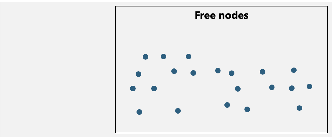
As a default, all nodes in the mesh are free nodes, meaning they are subject to updates in position due to smoothing.

• Free nodes

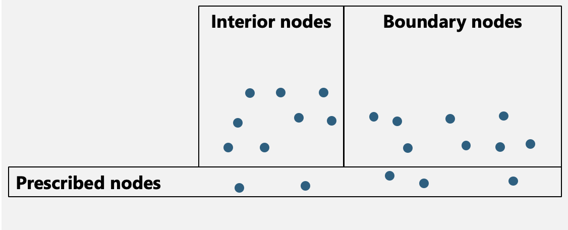
For the purpose of hierarchical smoothing, we categorize all nodes as belonging to one of the following categories.

• Boundary nodes
  • Nodes on the exterior of the domain and nodes that lie at the interface of two different blocks are reclassified from free nodes to boundary nodes.
  • Like free nodes, these nodes are also subject to updates in position due to smoothing.
  • Unlike free nodes, which are influenced by positions of neighboring nodes of any category, boundary nodes are only influenced positions of other boundary nodes, or prescribed nodes (described below).
• Interior nodes
  • The free nodes not categorized as boundary nodes are categorized as interior nodes.
  • Interior nodes are influenced by neighboring nodes of all categories.
• Prescribed nodes
  • Finally, we may wish to select nodes, typically but not necessarily from boundary nodes, to move to a specific location, often to match the desired shape of a mesh. These nodes are reclassified as prescribed nodes.
  • Prescribed nodes are not subject to updates in position due to smoothing because they are a priori prescribed to reside at a given location.

This classification is shown below in figures. All nodes in the mesh are categorized as FREE nodes:

Nodes that lie on the exterior and/or an interface are categoried as BOUNDARY nodes. The remaining free nodes that are not BOUNDARY nodes are INTERIOR nodes.

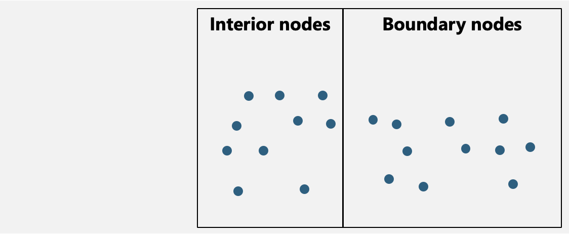
Some INTERIOR and BOUNDARY nodes may be recategorized as PRESCRIBED nodes.

The Hierarchy enum

These three categories, INTERIOR, BOUNDARY, and PRESCRIBED, compose the hierarchical structure of hierarchical smoothing. Nodes are classified in code with the following enum,

class Hierarchy(Enum):
    """All nodes must be categorized as beloning to one, and only one,
    of the following hierarchical categories.
    """

    INTERIOR = 0
    BOUNDARY = 1
    PRESCRIBED = 2

Hierarchical Control

Hierarchical control classifies all nodes in a mesh as belonging to a interior $\mathbb{A}$, boundary $\mathbb{B}$, or prescribed $\mathbb{C}$. These categories are mutually exclusive. Any and all nodes must belong to one, and only one, of these three categories. For a given node $\mathbf{p}$, let

• the set of interior neighbors be denoted ${\mathbf{q}}_{\mathbb{A}}$,
• the set of boundary neighbors be denoted ${\mathbf{q}}_{\mathbb{B}}$, and
• the set of prescribed neighbors be denoted ${\mathbf{q}}_{\mathbb{C}}$.

Hierarchical control redefines a node's neighborhood according to the following hierarchical rules:

• for any interior node $\mathbf{p}\in \mathbb{A}$, nodes ${\mathbf{q}}_{\mathbb{A}}$, ${\mathbf{q}}_{\mathbb{B}}$, and ${\mathbf{q}}_{\mathbb{C}}$ are neighbors; there is no change in the neighborhood,
• for any boundary node $\mathbf{p}\in \mathbb{B}$, only boundary nodes ${\mathbf{q}}_{\mathbb{B}}$ and prescribed nodes ${\mathbf{q}}_{\mathbb{C}}$ are neighbors; a boundary node neighborhood exludes interior nodes, and
• for any prescribed node $\mathbf{p}\in \mathbb{C}$, all neighbors of any category are excluded; the prescribed node's position does not change during smoothing.

The following figure shows this concept:

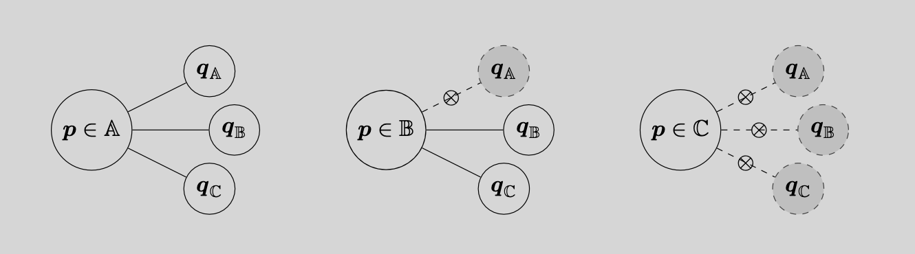
Figure: Classification of nodes into categories of interior nodes $\mathbb{A}$, boundary nodes $\mathbb{B}$, and prescribed nodes $\mathbb{C}$. Hierarchical relationship: An interior node's smooothing neighbors are nodes of any category, a boundary node's smoothing neighbors are other boundary nodes or other prescribed nodes, and prescribed nodes have no smoothing neighbors.

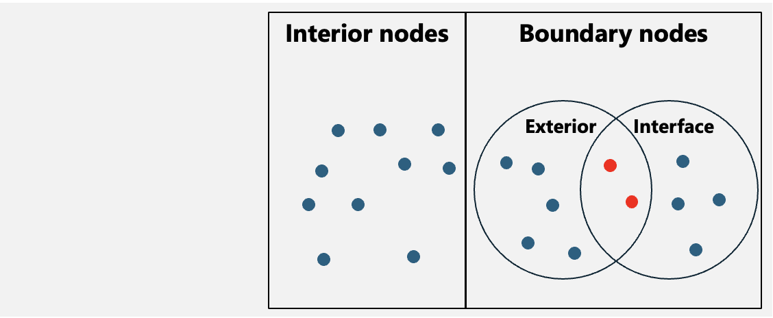
Relationship to a SideSet

A SideSet is a set of nodes on the boundary of a domain, used to prescribe a boundary condition on the finite element mesh.

• A subset of nodes on the boundary nodes is classified as exterior nodes.
• A different subset of nodes on the boundary is classified as interface nodes.
• A SideSet is composed of either exterior nodes or interface nodes.
• Because a node can lie both on the exterior and on an interface, some nodes (shown in red) are included in both the exterior nodes and the interface nodes.

Chen Example

Chen⁴ used medical image voxel data to create a structured hexahedral mesh. They noded that the approach generated a mesh with "jagged edges on mesh surface and material interfaces," which can cause numerical artifacts.

Chen used hierarchical Taubin mesh smoothing for eight (8) iterations, with $\lambda =0.6307$ and $\mu =-0.6732$ to smooth the outer and inner surfaces of the mesh.

References