Laplace Smoothing
Double X
We examine the most basic type of smoothing, Laplace smoothing, , without hierarchical control, with the Double X example.
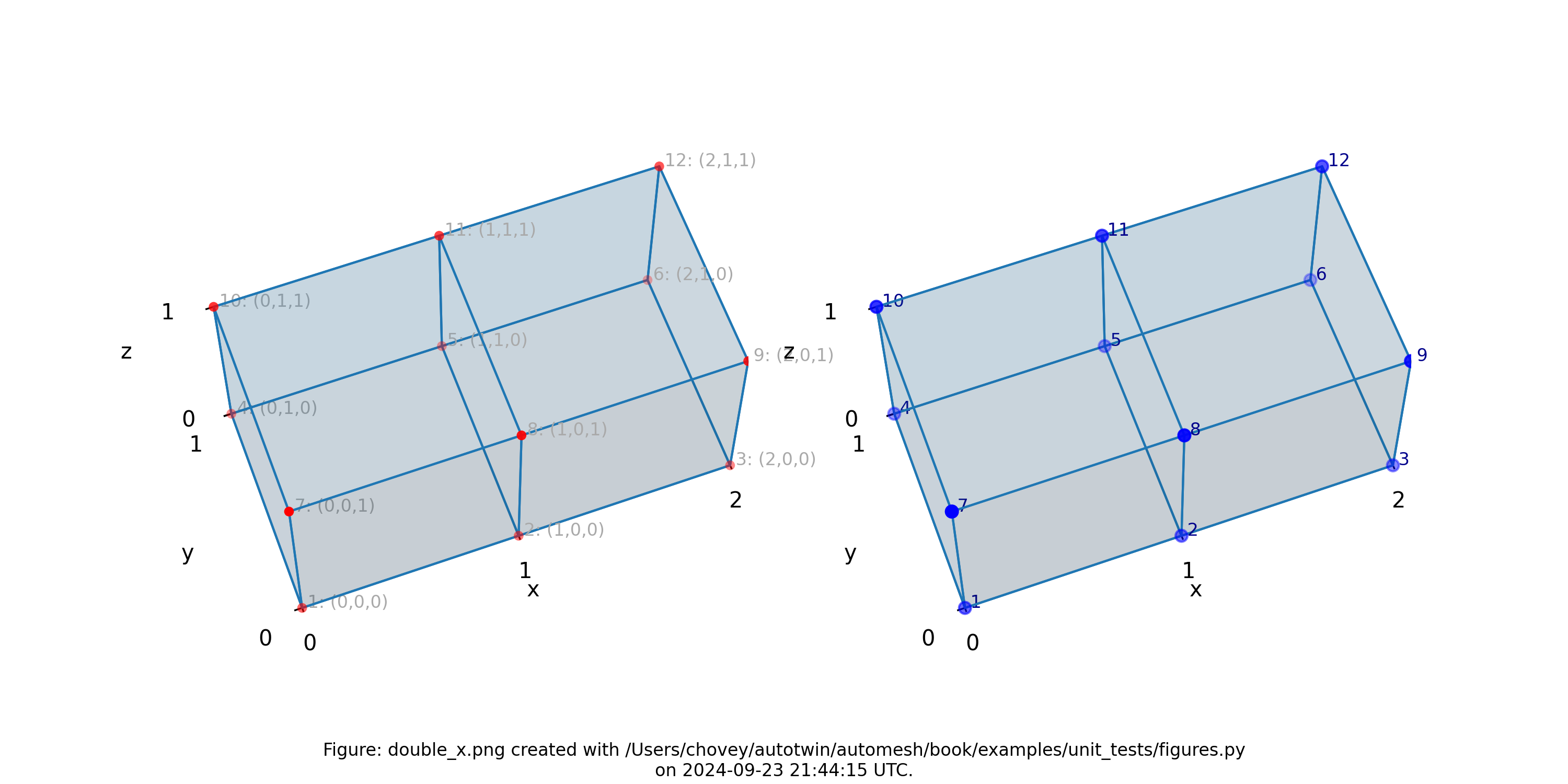
Figure: The Double X two-element example.
Table. The neighborhoods table. A node, with its neighbors, is considered a single neighborhood. The table has twelve neighborhoods.
| node | node neighbors |
|---|---|
| 1 | 2, 4, 7 |
| 2 | 1, 3, 5, 8 |
| 3 | 2, 6, 9 |
| 4 | 1, 5, 10 |
| 5 | 2, 4, 6, 11 |
| 6 | 3, 5, 12 |
| 7 | 1, 8, 10 |
| 8 | 2, 7, 9, 11 |
| 9 | 3, 8, 12 |
| 10 | 4, 7, 11 |
| 11 | 5, 8, 10, 12 |
| 12 | 6, 9, 11 |
Hierarchy
Following is a test where all nodes are BOUNDARY from the Hierarchy enum.
node_hierarchy: NodeHierarchy = (
    Hierarchy.BOUNDARY,
    Hierarchy.BOUNDARY,
    Hierarchy.BOUNDARY,
    Hierarchy.BOUNDARY,
    Hierarchy.BOUNDARY,
    Hierarchy.BOUNDARY,
    Hierarchy.BOUNDARY,
    Hierarchy.BOUNDARY,
    Hierarchy.BOUNDARY,
    Hierarchy.BOUNDARY,
    Hierarchy.BOUNDARY,
    Hierarchy.BOUNDARY,
)
Since there are no
INTERIORnodes norPRESCRIBEDnodes, the effect of hiearchical smoothing is nill, and the same effect would be observed were all nodes categorized asINTERIORnodes.
Iteration 1
Table: The smoothed configuration (x, y, z) after one iteration of Laplace smoothing.
| node | x | y | z |
|---|---|---|---|
| 1 | 0.1 | 0.1 | 0.1 |
| 2 | 1.0 | 0.075 | 0.075 |
| 3 | 1.9 | 0.1 | 0.1 |
| 4 | 0.1 | 0.9 | 0.1 |
| 5 | 1.0 | 0.925 | 0.075 |
| 6 | 1.9 | 0.9 | 0.1 |
| 7 | 0.1 | 0.1 | 0.9 |
| 8 | 1.0 | 0.075 | 0.925 |
| 9 | 1.9 | 0.1 | 0.9 |
| 10 | 0.1 | 0.9 | 0.9 |
| 11 | 1.0 | 0.925 | 0.925 |
| 12 | 1.9 | 0.9 | 0.9 |
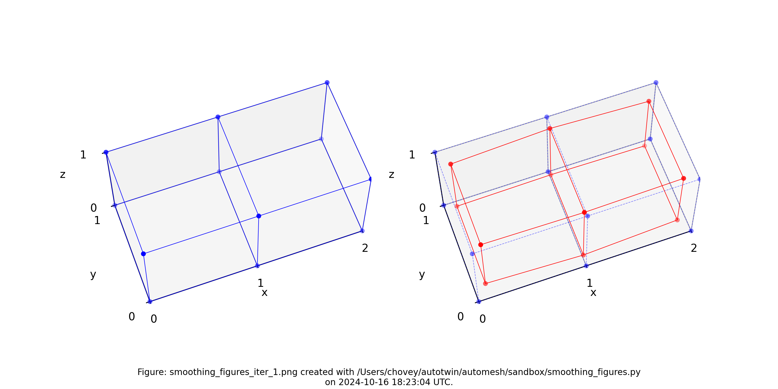
Figure: Two element test problem (left) original configuration, (right) subject to one iteration of Laplace smoothing.
Iteration 2
| node | x | y | z |
|---|---|---|---|
| 1 | 0.19 | 0.1775 | 0.1775 |
| 2 | 1.0 | 0.1425 | 0.1425 |
| 3 | 1.81 | 0.1775 | 0.1775 |
| 4 | 0.19 | 0.8225 | 0.1775 |
| 5 | 1.0 | 0.8575 | 0.1425 |
| 6 | 1.81 | 0.8225 | 0.1775 |
| 7 | 0.19 | 0.1775 | 0.8225 |
| 8 | 1.0 | 0.1425 | 0.8575 |
| 9 | 1.81 | 0.1775 | 0.8225 |
| 10 | 0.19 | 0.8225 | 0.8225 |
| 11 | 1.0 | 0.8575 | 0.8575 |
| 12 | 1.81 | 0.8225 | 0.8225 |
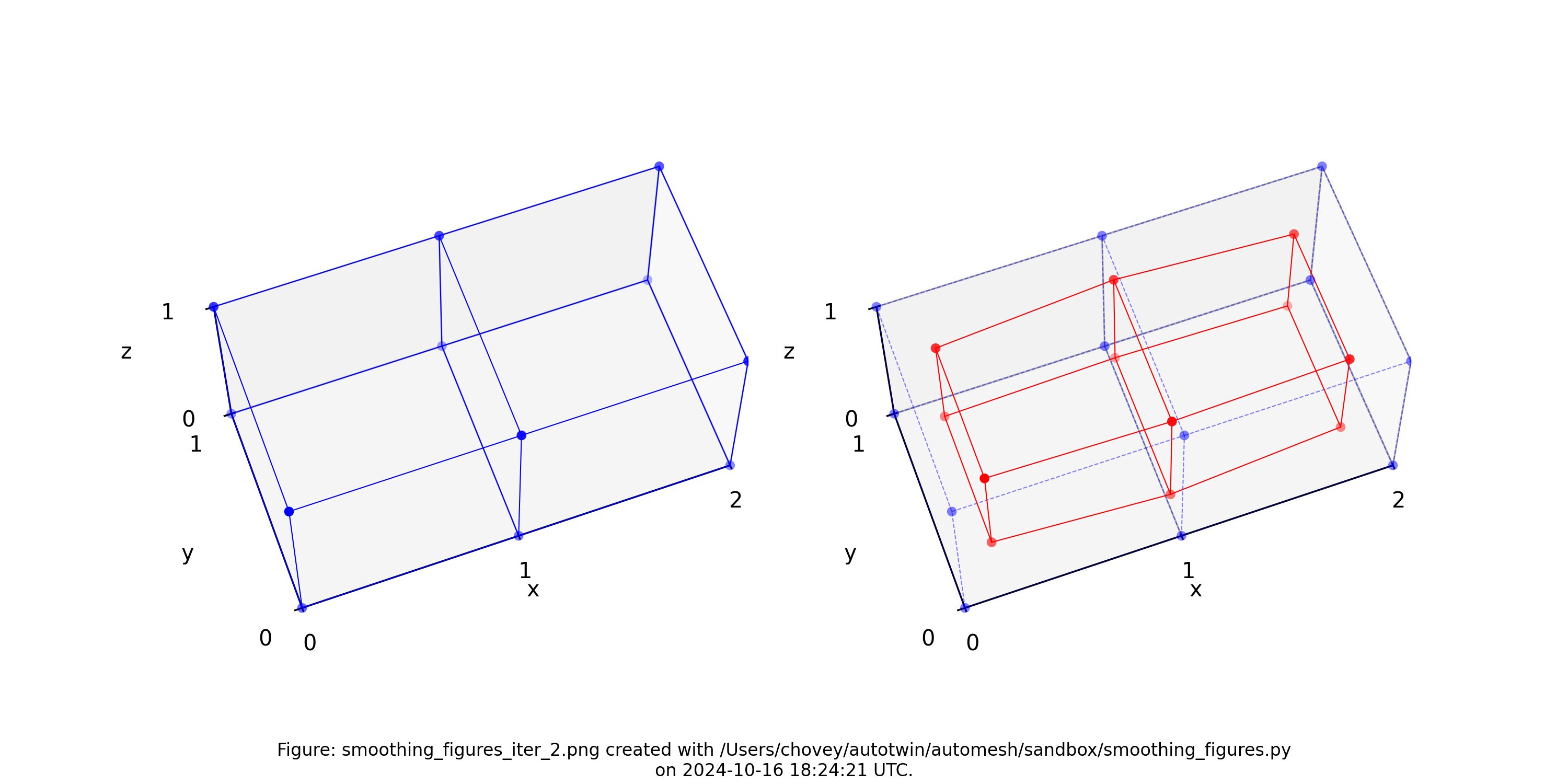
Figure: Two element test problem (left) original configuration, (right) subject to two iterations of Laplace smoothing.
Iteration 100
A known drawback of Laplace smoothing is that it can fail to preserve volumes. In the limit, volumes get reduced to a point, as illustrated in the figure below.
Figure: Two element test problem (left) original configuration, (right) subject to [1, 2, 3, 4, 5, 10, 20, 30, 100 iterations of Laplace smoothing. Animation created with Ezgif.