Hexahedral Metrics

automesh metrics hex --help
Quality metrics for an all-hexahedral finite element mesh

Usage: automesh metrics hex [OPTIONS] --input <FILE> --output <FILE>

Options:
  -i, --input <FILE>   Mesh input file (exo | inp | stl)
  -o, --output <FILE>  Quality metrics output file (csv | npy)
  -q, --quiet          Pass to quiet the terminal output
  -h, --help           Print help

automesh implements the following hexahedral element quality metrics¹:

• Maximum edge ratio ${\mathrm{ER}}_{\max }$
• Minimum scaled Jacobian ${\hat{J}}_{\min }$
• Maximum skew
• Element volume

A brief description of each metric follows.

Maximum Edge Ratio

• ${\mathrm{ER}}_{\max }$ measures the ratio of the longest edge to the shortest edge in a mesh element.
• A ratio of 1.0 indicates perfect element quality, whereas a very large ratio indicates bad element quality.
• Knupp et al.¹ (page 87) indicate an acceptable range of [1.0, 1.3].

Minimum Scaled Jacobian

• ${\hat{J}}_{\min }$ evaluates the determinant of the Jacobian matrix at each of the corners nodes, normalized by the corresponding edge lengths, and returns the minimum value of those evaluations.
• Interpretation
  • ${\hat{J}}_{\min }=1.0$: Perfect rectangular element
  • ${\hat{J}}_{\min }>0$: Element is valid (positive Jacobian)
  • ${\hat{J}}_{\min }=0$: Element zero volume
  • ${\hat{J}}_{\min }<0$: Invalid element (inverted/negative Jacobian)

Typically, mesh quality requirements specify ${\hat{J}}_{\min }>0.3$ for acceptable elements.

• Knupp et al.¹ (page 92) indicate an acceptable range of [0.5, 1.0], though in practice, minimum values as low as 0.2 and 0.3 are often used.

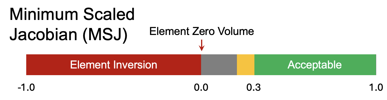
Figure. Illustration of minimum scaled Jacobian² with acceptable range [0.3, 1.0].

Maximum Skew

• Skew measures how much an element deviates from being a regular shape (e.g., in 3D, a cube or regular tetrahedron; in 2D, a square or equilateral triangle). A skew value of 0 indicates a perfectly regular shape, while higher values indicate increasing levels of distortion.
• Knupp et al.¹ (page 97) indicate an acceptable range of [0.0, 0.5].

Element Volume

• Measures the volume of the element.

Unit Tests

Inspired by Figure 2 of Livesu et al.³ reproduced here below

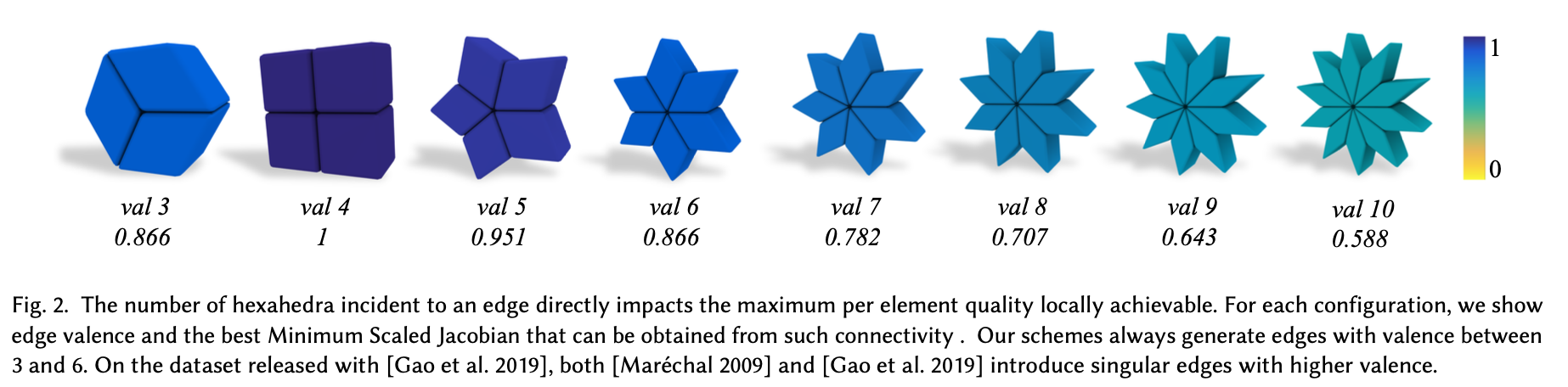
we examine several unit test singleton elements and their metrics.

valence	singleton	${\mathrm{ER}}_{\max }$	${\hat{J}}_{\min }$	$\mathrm{ske}{\mathrm{w}}_{\max }$	volume
3		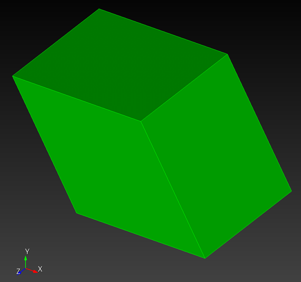1.000000e0 (1.000)	8.660253e-1 (0.866)	5.000002e-1 (0.500)	8.660250e-1 (0.866)
3' (noised)		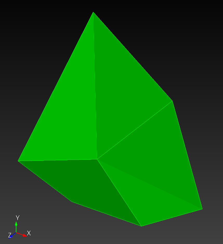1.292260e0 (2.325) ** Cubit (aspect ratio): 1.292	1.917367e-1 (0.192)	6.797483e-1 (0.680)	1.247800e0 (1.248)
4		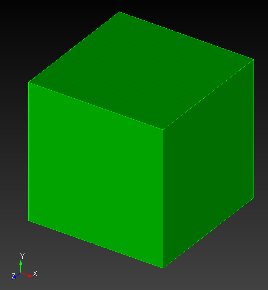1.000000e0 (1.000)	1.000000e0 (1.000)	0.000000e0 (0.000)	1.000000e0 (1.000)
4' (noised)		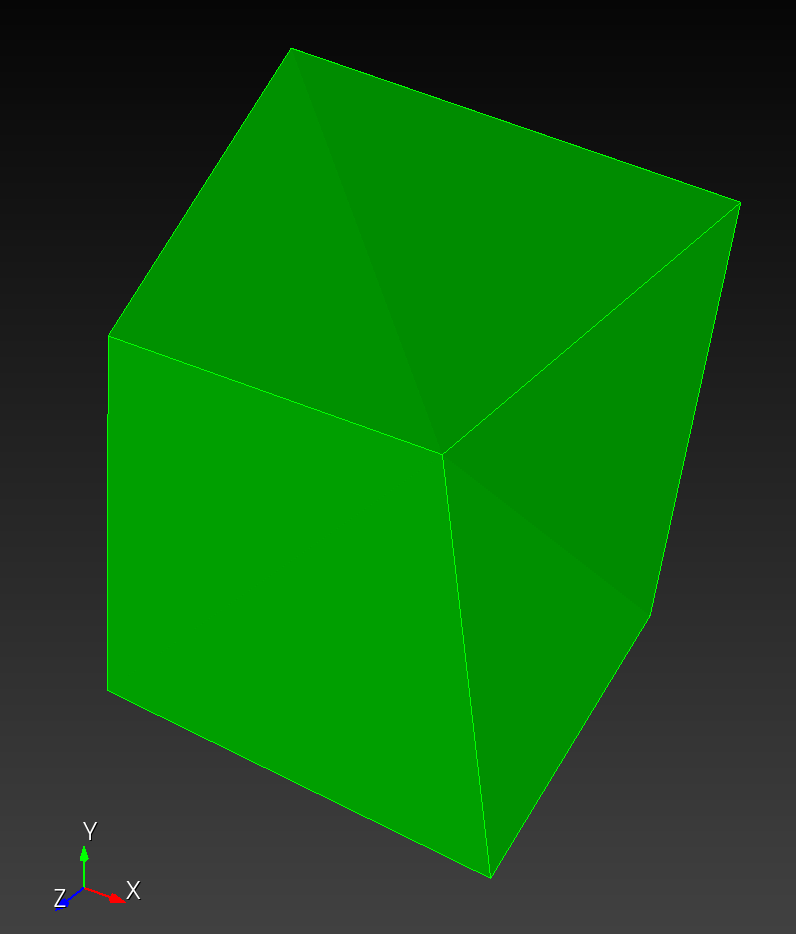1.167884e0 (1.727) ** Cubit (aspect ratio): 1.168	3.743932e-1 (0.374)	4.864936e-1 (0.486)	9.844008e-1 (0.984)
5		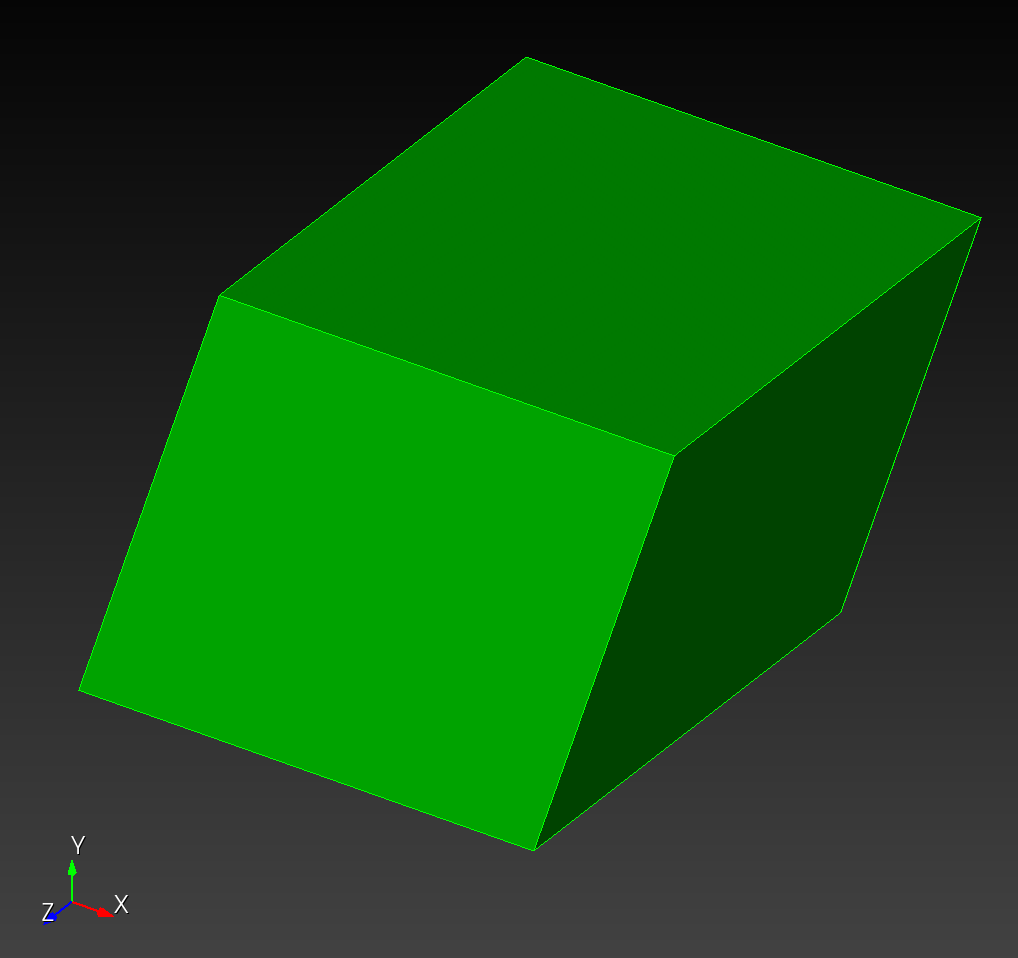1.000000e0 (1.000)	9.510566e-1 (0.951)	3.090169e-1 (0.309)	9.510570e-1 (0.951)
6		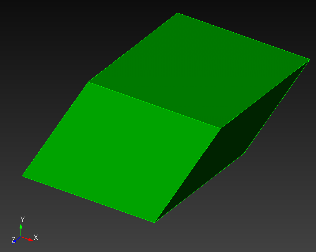1.000000e0 (1.000)	8.660253e-1 (0.866)	5.000002e-1 (0.500)	8.660250e-1 (0.866)
...	...	...	...	...	...
10		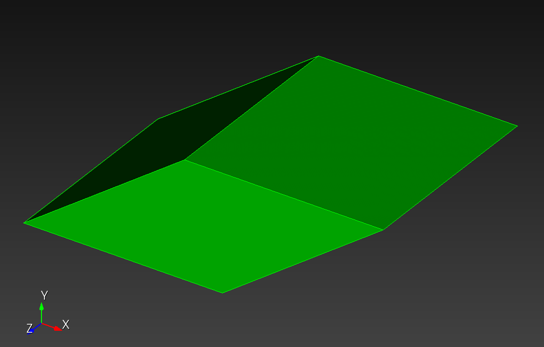1.000000e0 (1.000)	5.877851e-1 (0.588)	8.090171e-1 (0.809)	5.877850e-1 (0.588)

Figure: Hexahedral metrics. Leading values are from automesh. Values in parenthesis are results from HexaLab.⁴ Items with ** indicate where automesh and Cubit agree, but HexaLab disagrees. Cubit uses the term Aspect Ratio for Edge Ratio for hexahedral elements. All values were also verified with Cubit.

The connectivity for all elements:

1,    2,    4,    3,    5,    6,    8,    7

with prototype:

The element coordinates follow:

# 3
    1,      0.000000e0,      0.000000e0,      0.000000e0
    2,      1.000000e0,      0.000000e0,      0.000000e0
    3,     -0.500000e0,      0.866025e0,      0.000000e0
    4,      0.500000e0,      0.866025e0,      0.000000e0
    5,      0.000000e0,      0.000000e0,      1.000000e0
    6,      1.000000e0,      0.000000e0,      1.000000e0
    7,     -0.500000e0,      0.866025e0,      1.000000e0
    8,      0.500000e0,      0.866025e0,      1.000000e0

# 3'
    1,      0.110000e0,      0.120000e0,     -0.130000e0
    2,      1.200000e0,     -0.200000e0,      0.000000e0
    3,     -0.500000e0,      1.866025e0,     -0.200000e0
    4,      0.500000e0,      0.866025e0,     -0.400000e0
    5,      0.000000e0,      0.000000e0,      1.000000e0
    6,      1.000000e0,      0.000000e0,      1.000000e0
    7,     -0.500000e0,      0.600000e0,      1.400000e0
    8,      0.500000e0,      0.866025e0,      1.200000e0

# 4
    1,      0.000000e0,      0.000000e0,      0.000000e0
    2,      1.000000e0,      0.000000e0,      0.000000e0
    3,      0.000000e0,      1.000000e0,      0.000000e0
    4,      1.000000e0,      1.000000e0,      0.000000e0
    5,      0.000000e0,      0.000000e0,      1.000000e0
    6,      1.000000e0,      0.000000e0,      1.000000e0
    7,      0.000000e0,      1.000000e0,      1.000000e0
    8,      1.000000e0,      1.000000e0,      1.000000e0

# 4'
    1,      0.100000e0,      0.200000e0,      0.300000e0
    2,      1.200000e0,      0.300000e0,      0.400000e0
    3,     -0.200000e0,      1.200000e0,     -0.100000e0
    4,      1.030000e0,      1.102000e0,     -0.250000e0
    5,     -0.001000e0,     -0.021000e0,      1.002000e0
    6,      1.200000e0,     -0.100000e0,      1.100000e0
    7,      0.000000e0,      1.000000e0,      1.000000e0
    8,      1.010000e0,      1.020000e0,      1.030000e0

# 5
    1,      0.000000e0,      0.000000e0,      0.000000e0
    2,      1.000000e0,      0.000000e0,      0.000000e0
    3,      0.309017e0,      0.951057e0,      0.000000e0
    4,      1.309017e0,      0.951057e0,      0.000000e0
    5,      0.000000e0,      0.000000e0,      1.000000e0
    6,      1.000000e0,      0.000000e0,      1.000000e0
    7,      0.309017e0,      0.951057e0,      1.000000e0
    8,      1.309017e0,      0.951057e0,      1.000000e0

# 6
    1,      0.000000e0,      0.000000e0,      0.000000e0
    2,      1.000000e0,      0.000000e0,      0.000000e0
    3,      0.500000e0,      0.866025e0,      0.000000e0
    4,      1.500000e0,      0.866025e0,      0.000000e0
    5,      0.000000e0,      0.000000e0,      1.000000e0
    6,      1.000000e0,      0.000000e0,      1.000000e0
    7,      0.500000e0,      0.866025e0,      1.000000e0
    8,      1.500000e0,      0.866025e0,      1.000000e0

# 10
    1,      0.000000e0,      0.000000e0,      0.000000e0
    2,      1.000000e0,      0.000000e0,      0.000000e0
    3,      0.809017e0,      0.587785e0,      0.000000e0
    4,      1.809017e0,      0.587785e0,      0.000000e0
    5,      0.000000e0,      0.000000e0,      1.000000e0
    6,      1.000000e0,      0.000000e0,      1.000000e0
    7,      0.809017e0,      0.587785e0,      1.000000e0
    8,      1.809017e0,      0.587785e0,      1.000000e0

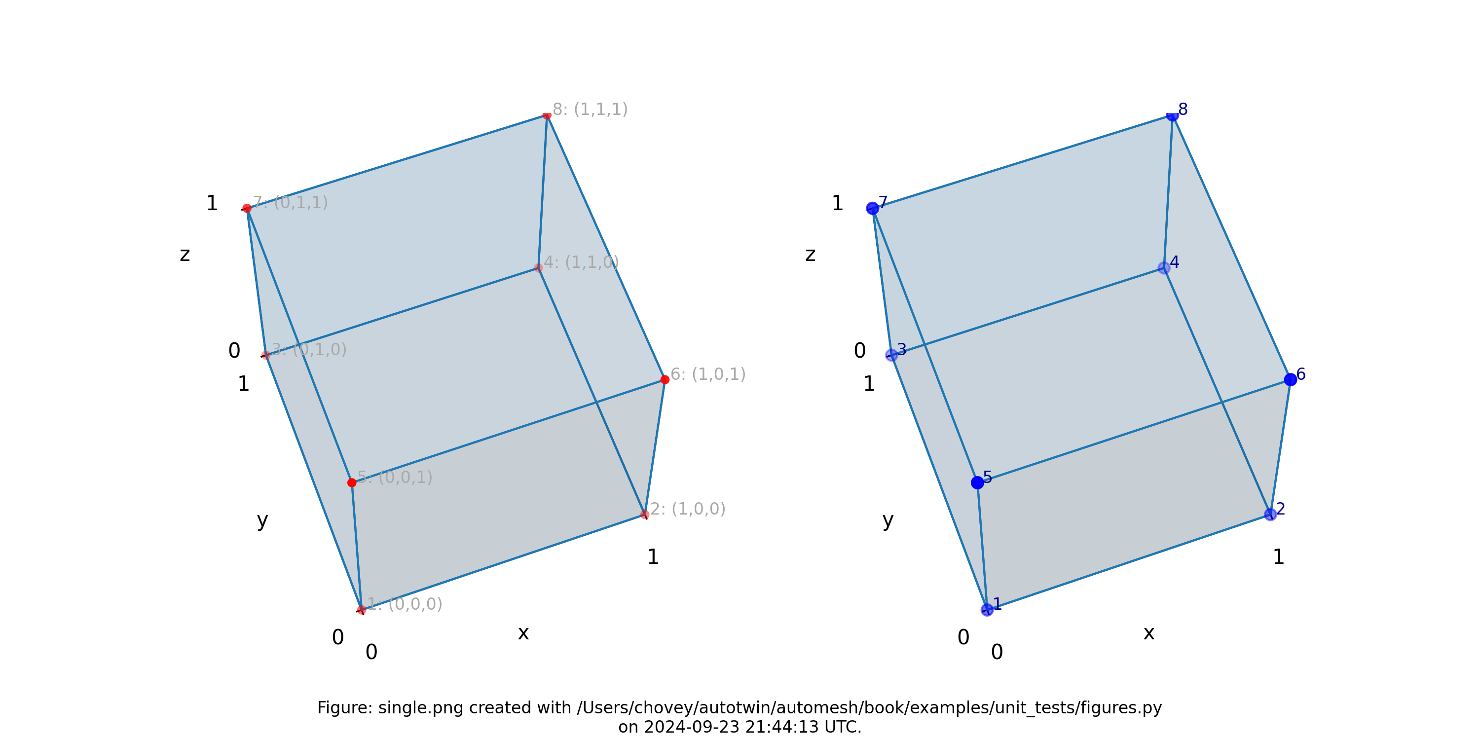
Local Numbering Scheme

Nodes

The local numbering scheme for nodes of a hexahedral element:

       7---------6
      /|        /|
     / |       / |
    4---------5  |
    |  3------|--2
    | /       | /
    |/        |/
    0---------1

Faces

From the exterior of the element, view the (0, 1, 5, 4) face and unwarp the remaining faces; the six face normals now point out of the page. The local numbering scheme for faces of a hexahedral element:

              7---------6
              |         |
              |    5    |
              |         |
    7---------4---------5---------6---------7
    |         |         |         |         |
    |    3    |    0    |    1    |    2    |
    |         |         |         |         |
    3---------0---------1---------2---------3
              |         |
              |    4    |
              |         |
              3---------2

${\hat{J}}_{\min }$ Formulation

For a hexahedral element with eight nodes, the scaled Jacobian at each node is computed as:

$$J_{\text{scaled}}:=\hat{J}=\frac{\mathbf{n}\cdot \mathbf{w}}{\Vert \mathbf{u}\Vert \Vert \mathbf{v}\Vert \Vert \mathbf{w}\Vert }\text{\hspace{1em}(1)}$$

where:

• $\mathbf{u}$, $\mathbf{v}$, and $\mathbf{w}$ are edge vectors emanating from the node,
• $\mathbf{n}=\mathbf{u}\times \mathbf{v}$ is the cross product of the first two edge vectors, and
• $\Vert \cdot \Vert$ denotes the Euclidean norm.

The minimum scaled Jacobian for the element is:

$${\hat{J}}_{\text{min}}:=\min \{{\hat{J}}^{(i)}{\}}_{i=0}^7\text{\hspace{1em}(2)}$$

Node Numbering Convention

The hexahedral element uses the following local node numbering (standard convention):

       7----------6
      /|         /|
     / |        / |
    4----------5  |
    |  |       |  |
    |  3-------|--2
    | /        | /
    |/         |/
    0----------1

Edge Vectors at Each Node

For each node $i$, three edge vectors are defined that point to adjacent nodes. The connectivity follows this pattern:

where ${\mathbf{x}}_i$ is the position of node $i$.

Algorithm

1. For each element in the mesh:

   a. Extract the 8 node indices from the connectivity array

   b. For each node $i\in \{0,1,\dots ,7\}$:

   • Compute edge vectors: $$\mathbf{u}={\mathbf{x}}_j-{\mathbf{x}}_i\text{\hspace{1em}(3)}$$ $$\mathbf{v}={\mathbf{x}}_k-{\mathbf{x}}_i\text{\hspace{1em}(4)}$$ $$\mathbf{w}={\mathbf{x}}_{\ell }-{\mathbf{x}}_i\text{\hspace{1em}(5)}$$ where $j$, $k$, $\ell$ are adjacent nodes per the table above

   • Compute cross product: $$\mathbf{n}=\mathbf{u}\times \mathbf{v}\text{\hspace{1em}(6)}$$

   • Compute scaled Jacobian: $${\hat{J}}^{(i)}=\frac{\mathbf{n}\cdot \mathbf{w}}{\Vert \mathbf{u}\Vert \Vert \mathbf{v}\Vert \Vert \mathbf{w}\Vert }\text{\hspace{1em}(7)}$$

   c. Take minimum over all 8 nodes: $${\hat{J}}_{\min }=\min \{{\hat{J}}^{(i)}{\}}_{i=0}^7\text{\hspace{1em}(8)}$$

2. Return the vector of minimum scaled Jacobians, one per element

Implementation

This prototyptical Rust implementation calculates the MSJ by evaluating the Jacobian at each of the eight corners using the edges connected to that corner.

#![allow(unused)]
fn main() {
struct Vector3 {
    x: f64,
    y: f64,
    z: f64,
}

impl Vector3 {
    fn sub(a: &Vector3, b: &Vector3) -> Vector3 {
        Vector3 { x: a.x - b.x, y: a.y - b.y, z: a.z - b.z }
    }

    fn dot(a: &Vector3, b: &Vector3) -> f64 {
        a.x * b.x + a.y * b.y + a.z * b.z
    }

    fn cross(a: &Vector3, b: &Vector3) -> Vector3 {
        Vector3 {
            x: a.y * b.z - a.z * b.y,
            y: a.z * b.x - a.x * b.z,
            z: a.x * b.y - a.y * b.x,
        }
    }

    fn norm(&self) -> f64 {
        (self.x.powi(2) + self.y.powi(2) + self.z.powi(2)).sqrt()
    }
}

/// Calculates the Minimum Scaled Jacobian for a hexahedron.
/// nodes: An array of 8 points ordered by standard FEM convention.
pub fn min_scaled_jacobian(nodes: &[Vector3; 8]) -> f64 {
    // Define the three edges meeting at each of the 8 corners
    // Corners are ordered: 0-3 (bottom face), 4-7 (top face)
    // For each node index: (current_node, u_target, v_target, w_target)
    let corner_indices = [
        (0, 1, 3, 4), // Corner 0: edges to 1, 3, 4
        (1, 2, 0, 5), // Corner 1: edges to 2, 0, 5
        (2, 3, 1, 6), // Corner 2: edges to 3, 1, 6
        (3, 0, 2, 7), // Corner 3: edges to 0, 2, 7
        (4, 7, 5, 0), // Corner 4: edges to 7, 5, 0
        (5, 4, 6, 1), // Corner 5: edges to 4, 6, 1
        (6, 5, 7, 2), // Corner 6: edges to 5, 7, 2
        (7, 6, 4, 3), // Corner 7: edges to 6, 4, 3
    ];

    let mut min_sj = f64::MAX;
    const EPSILON: f64 = 1e-15; // Small threshold to avoid division by zero

    for &(curr, i, j, k) in &corner_indices {
        // Calculate edge vectors: u, v, w from current node
        let u = Vector3::sub(&nodes[i], &nodes[curr]);
        let v = Vector3::sub(&nodes[j], &nodes[curr]);
        let w = Vector3::sub(&nodes[k], &nodes[curr]);

        // Calculate n = u × v
        let n = Vector3::cross(&u, &v);

        // Calculate scaled Jacobian: (n · w) / (||u|| * ||v|| * ||w||)
        let det = Vector3::dot(&n, &w);
        let lengths = u.norm() * v.norm() * w.norm();

        // Avoid division by zero for degenerate elements
        let sj = if lengths > EPSILON {
            det / lengths
        } else {
            f64::NEG_INFINITY // Flag completely degenerate elements
        };

        if sj < min_sj {
            min_sj = sj;
        }
    }

    min_sj
}
}

Implementation Notes

The implementation evaluates all 8 nodes of each element and returns the minimum value. This ensures that element distortion at any corner is captured, as poor quality at a single node can affect finite element solution accuracy.

Node-based ${\hat{J}}_{\min }$ Refinement

Node-based ${\hat{J}}_{\min }$ refinement reframes the traditional minimum scaled Jacobian formulation, which finds a per element minimum value, as a per node weighted value calculation.

• This calculation produces the incremental movement of the subject node that would improve the scaled Jacobian for the element at that node.
• The development follows an incremental update of nodal position, similar to the update formulation of Laplace and Taubin smoothing.)

Node and Element Valence

We define nodal valence as the number of nodes connected via an element edge to the subject node. For a hexahedral mesh, the minimum nodal valence is three (for a node at an external corner of an element); the maximum nodal valence eight (for a node on the internal portion of the mesh).

We define element valence as the number of elements connected via an element connectivity to the subject node. For a hexahedral mesh, the minimum element valence is one (for a node at an external corner of an element); the maximum nodal valence is eight (for a node on the internal portion of the mesh). Let $n_{\text{ev}}\subset [1,8]$ denote the element valence for a particular node.

For a given subject node with position $\mathbf{e}$ connected to one-to-eight elements, for the ${\ell }^{\text{th}}$ element, $\ell =0\dots n_{\text{ev}}-1$, find the three edge-connected element nodes, located at position $\mathbf{a},\mathbf{b}$, and $\mathbf{c}$. We assume the node numbering convention given above, with

$$\mathbf{u}:=\mathbf{a}-\mathbf{e}\text{\hspace{1em}(9)}$$ $$\mathbf{v}:=\mathbf{b}-\mathbf{e}\text{\hspace{1em}(10)}$$ $$\mathbf{w}:=\mathbf{c}-\mathbf{e}\text{\hspace{1em}(11)}$$

The current scaled Jacobian $\hat{J}$ is defined by the current location of $\mathbf{e}$, holding positions of $\mathbf{a},\mathbf{b}$, $\mathbf{c}$ constant:

$$\hat{J}:=\frac{\left[(\mathbf{a}-\mathbf{e})\times (\mathbf{b}-\mathbf{e})\right]\cdot (\mathbf{c}-\mathbf{e})}{\Vert \mathbf{a}-\mathbf{e}\Vert \Vert \mathbf{b}-\mathbf{e}\Vert \Vert \mathbf{c}-\mathbf{e}\Vert }\text{\hspace{1em}(12)}$$

From this definition, we define an ideal nodal position ${\mathbf{e}}^{\ast }$ that exactly produces a scaled Jacobian of unity:

$${\hat{J}}^{\ast }:=\frac{\left[(\mathbf{a}-{\mathbf{e}}^{\ast })\times (\mathbf{b}-{\mathbf{e}}^{\ast })\right]\cdot (\mathbf{c}-{\mathbf{e}}^{\ast })}{\Vert \mathbf{a}-{\mathbf{e}}^{\ast }\Vert \Vert \mathbf{b}-{\mathbf{e}}^{\ast }\Vert \Vert \mathbf{c}-{\mathbf{e}}^{\ast }\Vert }\stackrel{\text{set}}{=}1.0\text{\hspace{1em}(13)}$$

The ideal position ${\mathbf{e}}^{\ast }$ is a point such that the vectors $(\mathbf{a}-{\mathbf{e}}^{\ast })$, $(\mathbf{b}-{\mathbf{e}}^{\ast })$, and $(\mathbf{c}-{\mathbf{e}}^{\ast })$ are mutually orthogonal. How can we solve for ${\mathbf{e}}^{\ast }$ in terms of $\mathbf{a}$, $\mathbf{b}$, and $\mathbf{c}$?

We solve for ${\mathbf{e}}^{\ast }$ by assuring that the three right triangles formed by ${\mathbf{e}}^{\ast }$ and combinations of $\mathbf{a}$, $\mathbf{b}$, and $\mathbf{c}$ satisfy Pythagorean's theorem. Let lengths

$$u^{\ast }=\Vert {\mathbf{u}}^{\ast }\Vert =\Vert \mathbf{a}-{\mathbf{e}}^{\ast }\Vert \text{\hspace{1em}(14)}$$ $$v^{\ast }=\Vert {\mathbf{v}}^{\ast }\Vert =\Vert \mathbf{b}-{\mathbf{e}}^{\ast }\Vert \text{\hspace{1em}(15)}$$ $$w^{\ast }=\Vert {\mathbf{w}}^{\ast }\Vert =\Vert \mathbf{c}-{\mathbf{e}}^{\ast }\Vert \text{\hspace{1em}(16)}$$

Then Pythagorean's theorem requires

$$(u^{\ast }{)}^2+(v^{\ast }{)}^2=(\mathbf{b}-\mathbf{a})\cdot (\mathbf{b}-\mathbf{a})\text{\hspace{1em}(17)}$$ $$(v^{\ast }{)}^2+(w^{\ast }{)}^2=(\mathbf{c}-\mathbf{b})\cdot (\mathbf{c}-\mathbf{b})\text{\hspace{1em}(18)}$$ $$(w^{\ast }{)}^2+(u^{\ast }{)}^2=(\mathbf{a}-\mathbf{c})\cdot (\mathbf{a}-\mathbf{c})\text{\hspace{1em}(19)}$$

This represents a system of three independent equations and three unknowns $u^{\ast }$, $v^{\ast }$, and $w^{\ast }$.

Subtracting Eq. (18) from Eq. (17) and solving,

$$2(u^{\ast }{)}^2=(\mathbf{b}-\mathbf{a})\cdot (\mathbf{b}-\mathbf{a})-(\mathbf{c}-\mathbf{b})\cdot (\mathbf{c}-\mathbf{b})+(\mathbf{a}-\mathbf{c})\cdot (\mathbf{a}-\mathbf{c})\text{\hspace{1em}(20)}$$

Before proceeding, we can further simplify the expressions of these equations by defining edge vectors that connect each of the points $\mathbf{a}$, $\mathbf{b}$, and $\mathbf{c}$ that circle the path on $△ABC$. Let

$$\mathbf{r}:=\mathbf{b}-\mathbf{a}⟹r^2=(\mathbf{b}-\mathbf{a})\cdot (\mathbf{b}-\mathbf{a})=\Vert \mathbf{r}{\Vert }^2\text{\hspace{1em}(21)}$$ $$\mathbf{s}:=\mathbf{c}-\mathbf{b}⟹s^2=(\mathbf{c}-\mathbf{b})\cdot (\mathbf{c}-\mathbf{b})=\Vert \mathbf{s}{\Vert }^2\text{\hspace{1em}(22)}$$ $$\mathbf{t}:=\mathbf{a}-\mathbf{c}⟹t^2=(\mathbf{a}-\mathbf{a})\cdot (\mathbf{a}-\mathbf{c})=\Vert \mathbf{t}{\Vert }^2\text{\hspace{1em}(23)}$$

Note that the square values of each of the three hypotenuses is $r^2$, $s^2$, and $t^2$, respectively. Then

$$(u^{\ast }{)}^2+(v^{\ast }{)}^2=r^2\text{\hspace{1em}(24)}$$ $$(v^{\ast }{)}^2+(w^{\ast }{)}^2=s^2\text{\hspace{1em}(25)}$$ $$(w^{\ast }{)}^2+(u^{\ast }{)}^2=t^2\text{\hspace{1em}(26)}$$

Solving,

$$2(u^{\ast }{)}^2=r^2-s^2+t^2\text{\hspace{1em}(27)}$$ $$2(v^{\ast }{)}^2=s^2-t^2+r^2\text{\hspace{1em}(28)}$$ $$2(w^{\ast }{)}^2=t^2-r^2+s^2\text{\hspace{1em}(29)}$$

The lengths $u^{\ast }$, $v^{\ast }$, and $w^{\ast }$ are now known. It is also known that in the local $x$, $y$, $z$ coordinate system spanned by the right-handed, orthonormal triad ${\hat{\mathbf{u}}}^{\ast }$, ${\hat{\mathbf{v}}}^{\ast }$, ${\hat{\mathbf{w}}}^{\ast }$ at point ${\mathbf{e}}^{\ast }$, the lengths $u^{\ast }$, $v^{\ast }$, $w^{\ast }$, with their corresponding components of $\mathbf{a}$, $\mathbf{b}$, $\mathbf{c}$ define the three components of ${\mathbf{e}}^{\ast }$, that is,

$${\mathbf{e}}^{\ast }=\left\{\begin{array}{c}{e}_x^{\ast }\\ e_y^{\ast }\\ e_z^{\ast }\end{array}\right\}=\left\{\begin{array}{c}{a}_x-u^{\ast }\\ b_y-v^{\ast }\\ c_z-w^{\ast }\end{array}\right\}\text{\hspace{1em}(30)}$$

Weighting (aka Voting)

Any scheme for weighting of the connected elements can be adopted. Perhaps elements that lie on the surface should be given greater weighting than elements that lie on the interior. The effect would be to create higher quality element near the surface, and relatively lower quality element would be pushed into the interior of the volume. For a given element $\ell$ in the element valence of node $\mathbf{e}$, $\ell =0\dots n_{\text{ev}}-1$,

$${\mathbf{e}}^{\ast }=\sum _{\ell =0}^{n_{\text{ev}}-1}{w}_{\ell }{\mathbf{e}}_{\ell }^{\ast }/\sum _{\ell =0}^{n_{\text{ev}}-1}{w}_{\ell }\text{\hspace{1em}(31)}$$

For now, however, let's just explore the equal weighting scheme:

$${\mathbf{e}}^{\ast }=\sum _{\ell =0}^{n_{\text{ev}}-1}{\mathbf{e}}_{\ell }^{\ast }/n_{\text{ev}}\text{\hspace{1em}(32)}$$

This is just the average of all ideal locations for each connected element $\ell$.

Iteration

We define a gap vector $\Delta {\mathbf{e}}^{(k)}$ as originating at the current position ${\mathbf{e}}^{(k)}$ and terminating at the current ideal nodal position ${\mathbf{e}}^{\ast (k)}$:

$$\Delta {\mathbf{e}}^{(k)}:={\mathbf{e}}^{\ast (k)}-{\mathbf{e}}^{(k)}\text{\hspace{1em}(33)}$$

The quantity $\Delta {\mathbf{e}}^{(k)}$ is geometrically interpreted as a search direction or gap vector, analogous to the $\Delta \mathbf{p}$ gap vector defined for Laplace smoothing.

Let $\lambda \in {\mathbb{R}}^{+}$ be the positive scaling factor for the gap $\Delta {\mathbf{e}}^{(k)}$.

Since

$${\mathbf{e}}^{\ast (k)}={\mathbf{e}}^{(k)}+\lambda \Delta {\mathbf{e}}^{(k)}\mathrm{when}\lambda =1\text{\hspace{1em}(34)}$$

subdivision of this relationship into several substeps gives rise to an iterative approach. We typically select $\lambda <1$ to avoid overshoot of the update, $\lambda \in {\mathbb{R}}^{+}\subset (0,1)$.

At iteration $k$, we update the position of ${\mathbf{e}}^{(k)}$ by an amount $\lambda \Delta {\mathbf{e}}^{(k)}$ to ${\mathbf{e}}^{(k+1)}$ as

$${\mathbf{e}}^{(k+1)}:={\mathbf{e}}^{(k)}+\lambda \Delta {\mathbf{e}}^{(k)},\text{\hspace{1em}(35)}$$

with

$$\Delta {\mathbf{e}}^{(k)}={\mathbf{e}}^{\ast (k)}-{\mathbf{e}}^{(k)}.\text{\hspace{1em}(36)}$$

Thus

$${\mathbf{e}}^{(k+1)}:={\mathbf{e}}^{(k)}+\lambda \left(\Delta {\mathbf{e}}^{(k)}\right),\text{\hspace{1em}(37)}$$

$${\mathbf{e}}^{(k+1)}:={\mathbf{e}}^{(k)}+\lambda \left({\mathbf{e}}^{\ast (k)}-{\mathbf{e}}^{(k)}\right),\text{\hspace{1em}(38)}$$

and finally considering equal weighting for all connected elements

$$\boxed{{\mathbf{e}}^{(k+1)}:={\mathbf{e}}^{(k)}+\lambda \left(\sum _{\ell =0}^{n_{\text{ev}}-1}{\mathbf{e}}_{\ell }^{\ast (k)}/n_{\text{ev}}-{\mathbf{e}}^{(k)}\right).}\text{\hspace{1em}(39)}$$

Sign Check

Because the derivation of finding ${\mathbf{e}}^{\ast }$ involves squared terms, we must take one additional precaution to assure that the search direction $\Delta \mathbf{e}$ is opposite the direction of the face normal $\mathbf{n}$ of $△ABC$.

Let the face normal be defined as the cross product of any two edges of $△ABC$, e.g.,

$$\mathbf{n}:=\mathbf{r}\times \mathbf{s}\text{\hspace{1em}(40)}$$

In general, $\Delta \mathbf{e}$ and $\mathbf{n}$ are not colinear (they are colinear only for the special case where all lengths $r$, $s$, $t$ are equal). Nonetheless, for a non-inverted element with the search direction $\Delta \mathbf{e}$ in the opposite direction of the face normal $\mathbf{n}$, the sign function (sgn) is used,

$$\text{sgn}(\Delta \mathbf{e})=-\text{sgn}(\mathbf{n})\text{\hspace{1em}(41)}$$

If an inverted element is encountered such that $\text{sgn}(\Delta \mathbf{e})=\text{sgn}(\mathbf{n})$, then Eq. (39) should be modified to reverse the direction of $\Delta \mathbf{e}$, viz.

$$\boxed{{\mathbf{e}}^{(k+1)}:={\mathbf{e}}^{(k)}-\lambda \left(\sum _{\ell =0}^{n_{\text{ev}}-1}{\mathbf{e}}_{\ell }^{\ast (k)}/n_{\text{ev}}-{\mathbf{e}}^{(k)}\right).}\text{\hspace{1em}(42)}$$

Compare the $+\lambda$ in Eq. (39) to the $-\lambda$ in Eq. (42).

References

1. Knupp PM, Ernst CD, Thompson DC, Stimpson CJ, Pebay PP. The verdict geometric quality library. SAND2007-1751. Sandia National Laboratories (SNL), Albuquerque, NM, and Livermore, CA (United States); 2006 Mar 1. link ↩ ↩2 ↩3 ↩4

2. Hovey CB. Naval Force Health Protection Program Review 2023 Presentation Slides. SAND2023-05198PE. Sandia National Lab.(SNL-NM), Albuquerque, NM (United States); 2023 Jun 26. link ↩

3. Livesu M, Pitzalis L, Cherchi G. Optimal dual schemes for adaptive grid based hexmeshing. ACM Transactions on Graphics (TOG). 2021 Dec 6;41(2):1-4. link ↩

4. Bracci M, Tarini M, Pietroni N, Livesu M, Cignoni P. HexaLab.net: An online viewer for hexahedral meshes. Computer-Aided Design. 2019 May 1;110:24-36. link ↩